
Forecasting San Francisco Region Home Median Values (Part 2)
Photo by Business Insider
Programming Language: R
Exploratory Analyses, DotCom and Housing Bubble Impact: Part 1
After performing exploratory analysis on the Dotcom Bubble and Housing Bubble events that impacted the San Francisco region, we decided to split the dataset to evaluate the best forecasting model accordingly:
- Training set (1996 Q2 - 2016 Q4)
- Testing set (2017 Q1 - 2018 Q2)
1. Autoregressive Model (AR)
In an Autoregression model, we forecast the variable of interest using a linear combination of past values of the variable. The term autoregression indicates that it is a regression of the variable against itself.
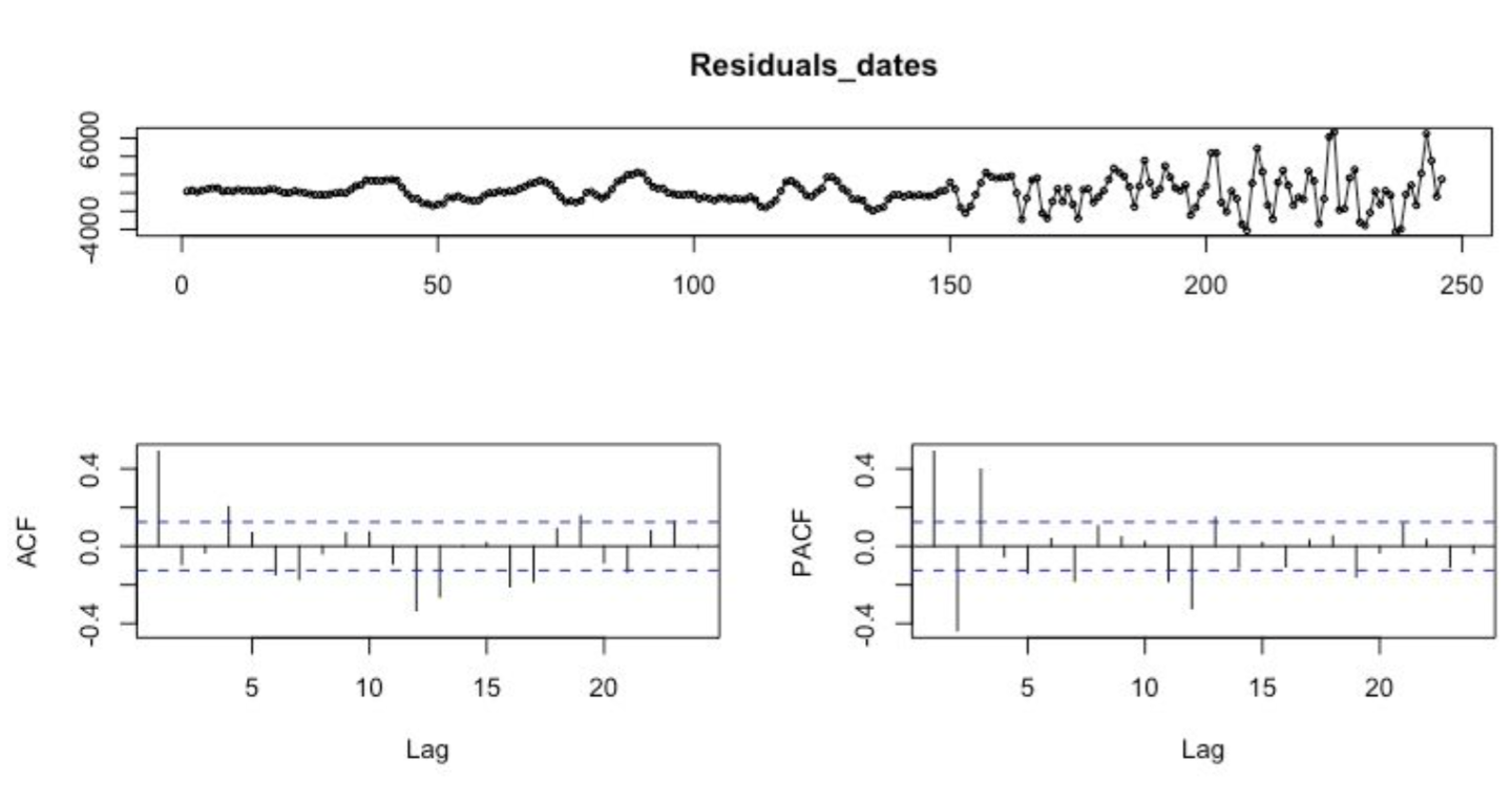
After building some features, we first ran a regression on the home Median Values using the training set then evaluated if whether or not the residuals were considered as white noise. We then plotted the autocorrelation function (ACF) and partial autocorrelation (PACF) plots of the differenced series using R where we tentatively identified the numbers of AR needed for the Autoregressive Model.
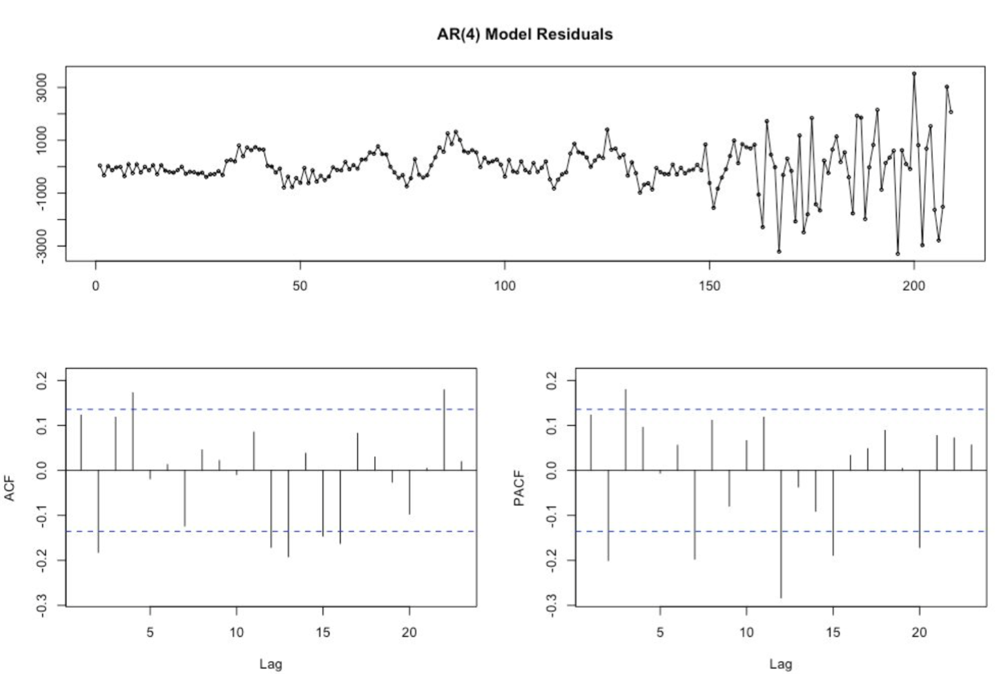
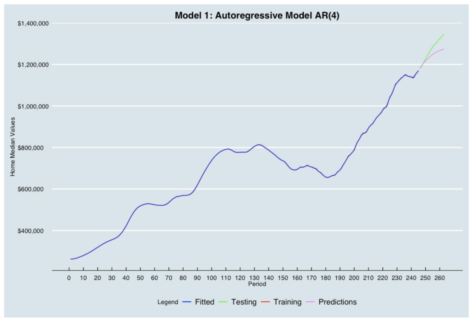
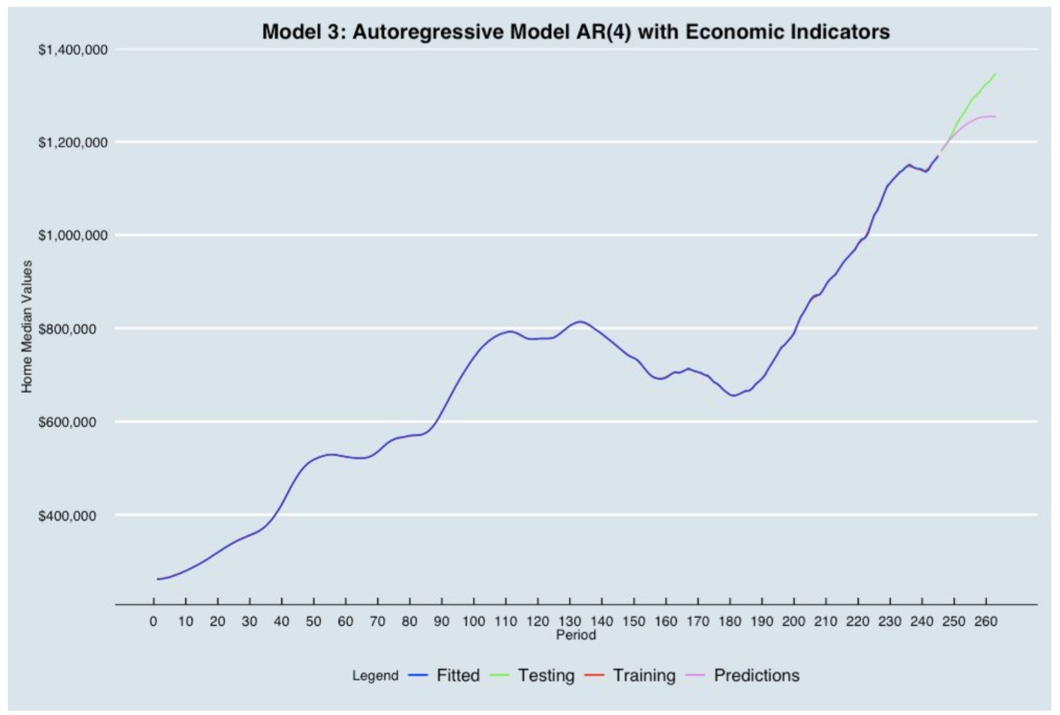
Based on the ACF and PACF, we built the Autoregressive Model of order 4 on the training set. We then incorporated a plot showing the training, fitted values, testing data and the predictions built from the AR(4) Model. The blue line (Fitted) matches perfectly the red line (training). The AR(4) model is underpredicting as the purple line (Predictions) is below the green line (Testing).
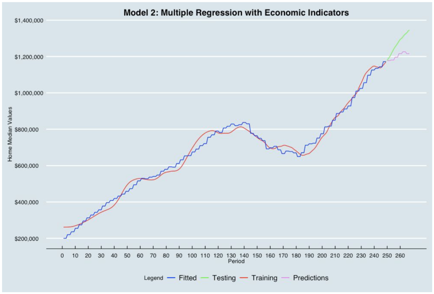
2. Multiple Regression Using Economic Indicators
In this case, the dependent variable is the home median values in San Francisco region. And the independent variables are the following economic indicators:
- Consumer Price Index (CPI)
- Housing Prices Indicator
- Producer Price Indices (PPI)
- Short-Term Interest Rates
- Unemployment Rate
- Real Gross Domestic Product (GDP)
- Disposable Personal Income (DPI)
The blue line (Fitted) does not quite match the red line (Training). The Multiple regression Model is underpredicting as the purple line (Predictions) is below the green line (Testing).
3. Combination of AR and Economic Indicators Modeling
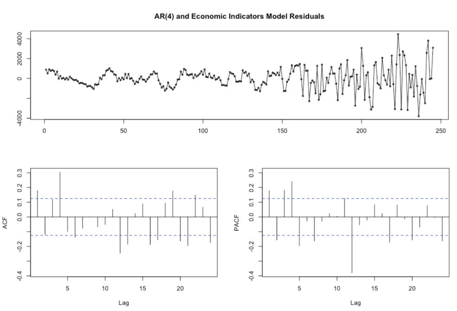
Following the definitions from Model 1 and Model 2, the combination model combines both the Autoregressive Model and the multiple regression model where we adjust estimated regression coefficients and standard errors when the errors have an AR structure.
We first ran a regression analysis to analyze the residuals in order to assess dependencies between the variables. Using the forecast library package in R, we plotted the ACF and PACF plot to identify the numbers of AR needed for the Autoregressive Model. We concluded that an order of lag 4 was required to build the Autoregressive model with the economic indicators. The final plot of residuals from the AR(4) and Multiple Regression Model shows no dependencies.
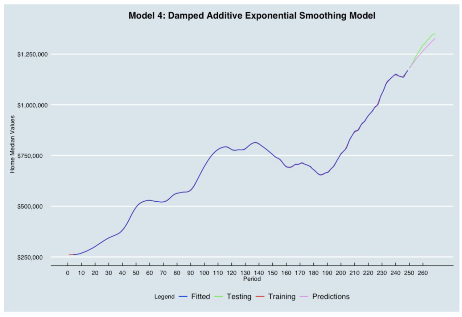
4. Damped Additive Trend Exponential Smoothing (Holt Methods- DATES)
The rationale behind damped trend model is based on past findings where the practice of projecting a straight line trend indefinitely into the future was often too optimistic (or pessimistic). Thus, an autoregressive parameter (phi) was added to modify the trend components in Holt’s linear trend method. If the data have a strong consistent trend, phi would be fitted at value near 1, and the forecast would be nearly the same as Holt’s method. However, if the data is extremely noisy or the trend is erratic, phi would be fitted to a value less than 1 to create a damped forecast function.
We found there are at least two special events (the dotcom and Housing Bubble) in our dataset that make the trend somewhat erratic. Therefore, we decided to forecast future data using the DATES model in Exponential Smoothing Macro (ESM) with the following optimized parameters (any number between 0 and 1).
- alpha (smoothing parameter for the level component of the forecast) = 1
- beta (smoothing parameter for the trend component of the forecast) = 1
- gamma (smoothing parameter for the seasonality component of the forecast) = 0
- phi (damping parameter)= 0.9
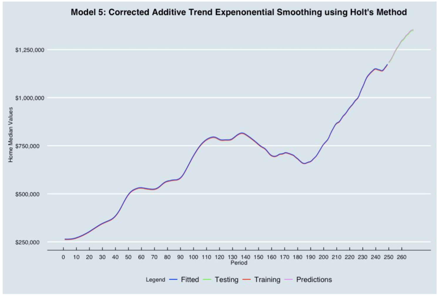
5. Corrected Additive Trend Exponential Smoothing (Holt Methods - CATES)
The Exponential Smoothing method is a time series model that schemes weight past observations using exponentially decreasing weights. In other words, recent observations are given relatively more weight in forecasting than the older observations. By definition, the corrected Additive Trend Exponential Smoothing is a simple exponential smoothing that eliminates the lag by estimating the magnitude trend and giving the necessary corrections to the forecast model.
In order determine the systematic component, we analyzed the graph and found that there was an increasing trend but no seasonality. The Corrected Additive Trend Exponential Smoothing is a good forecasting method to solve this problem. We first performed a regression analysis on the home median values data to find the trend and the level at period 0. Secondly, we applied the Corrected Trend Smoothing Exponential forecast formula to compute the prediction on the training data. Finally, we optimized the parameters 𝞪 and 𝛃 in order to minimize the training RMSE:
- alpha = 0.958
- beta = 0.0045
6. ARIMA Model
ARIMA is an acronym that stands for Autoregressive Integrated Moving Average. This model is a popular and widely used statistical method in time-series forecasting. Each of the components is specified in the model as a parameter. A standard notation ARIMA(p,d,q) is used which indicates the specific ARIMA model being used.
The ARIMA model parameters are defined below:
- p: The number of lag observations included in the model
- d: The number of times that the raw observations are differenced
- q: The size of moving average window
We used the auto.arima function in R because it returns the best ARIMA model according to either the AIC, AICc and BIC. The function conducts a search over each possible model within the order constraints provided. Before fitting the model, we converted the data frame format to a time-series data format using the ts() function. We defined the size of training and testing, divided the data into training and testing set using window() function, fitted the training set using auto.arima function and generated the forecasts.
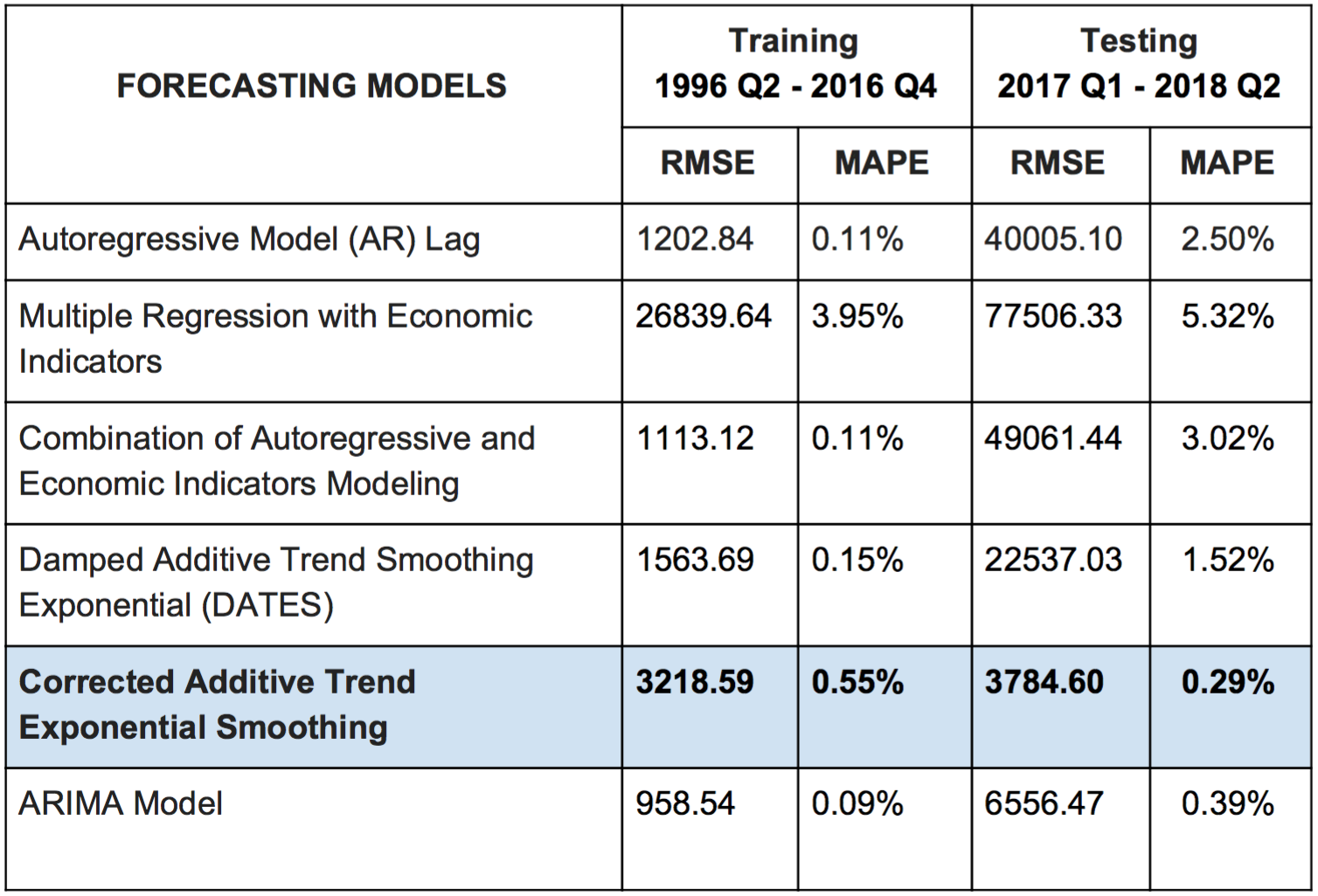
Evaluation of The Forecasting Models
The training set is used to estimate any parameters of a forecasting method and the test set is used to evaluate its accuracy. In evaluating a forecast models accuracy, the two most commonly used scale-dependent measures are:
- MAPE (Mean Absolute Percentage Error)
- RMSE (Root Mean Square Error)
The MAPE tells us how big of an error we can expect from the forecast of San Francisco region Home Median values on average in percentage, while the RMSE tells us about the difference between the predicted and actual values of San Francisco Home Median.
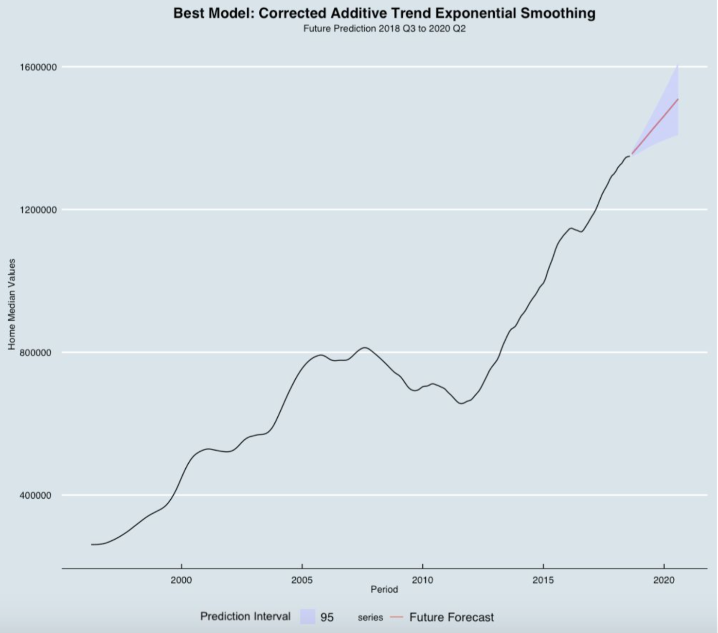
Based on the testing MAPE and testing RMSE, the best forecasting model for future predictions is the Corrected Additive Trend Exponential Smoothing Model (Holt Methods - CATES).
Best Model Predictions (2018 - 2020)
The prediction interval gives an interval within which we expect the home median values in San Francisco to lie with a specified probability. The prediction interval range values calculated from the table above are able to tell us how much uncertainty is associated with each forecast. In the plot above, we can see the blue range (Prediction Interval) as a 95% prediction interval that contains a range of values which should include the actual future value with probability 95%. The red lines (Future Forecast) falls in between the lower and upper bound of the prediction interval. We applied our best model to predict home median value in a 2 years forecast horizon (September 2018 - August 2020). Using our best model (Corrected Additive Trend Exponential Smoothing), the average home median value in 2019 would be over $1.4 million.