

New York Property Fraud Detection Using Unsupervised Models
Photo by Zillow
Programming Language: R and SQL
Project Goal
The primary objective of our analysis is to identify potential fraudulent instances in the New York property valuation data by building unsupervised models, and to conduct further investigation on the flagged records.
Data Source and Dictionary
The City of New York Property a Valuation and Assessment Data file is a public available dataset provided by the Department of Finance (DOF) on the City of New York Open Data website. The dataset contains the records of more than 1 million properties across the City of New York and information on their owners, building classes, tax classes sizes, assessment values, addresses, zip code, etc.
Exploratory Data Analyses (EDA)
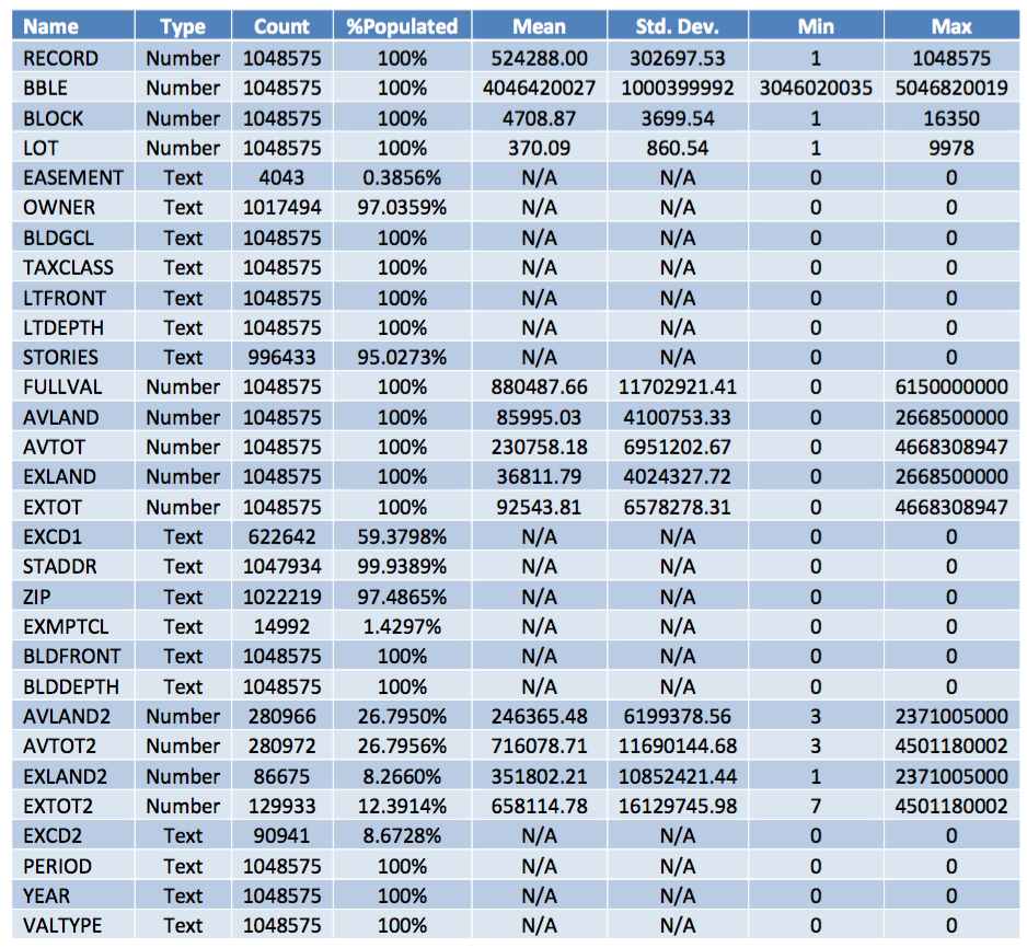
The City of New York Property Valuation and Assessment dataset contains a total of 1,048,575 records (rows) with 30 variables (columns). Among the 30 variables, 13 are categorical variables, 14 numeric variables, 2 text variables, and 1 date variable. All the records are from November 2011. Below is a summary of all the variables in the dataset.
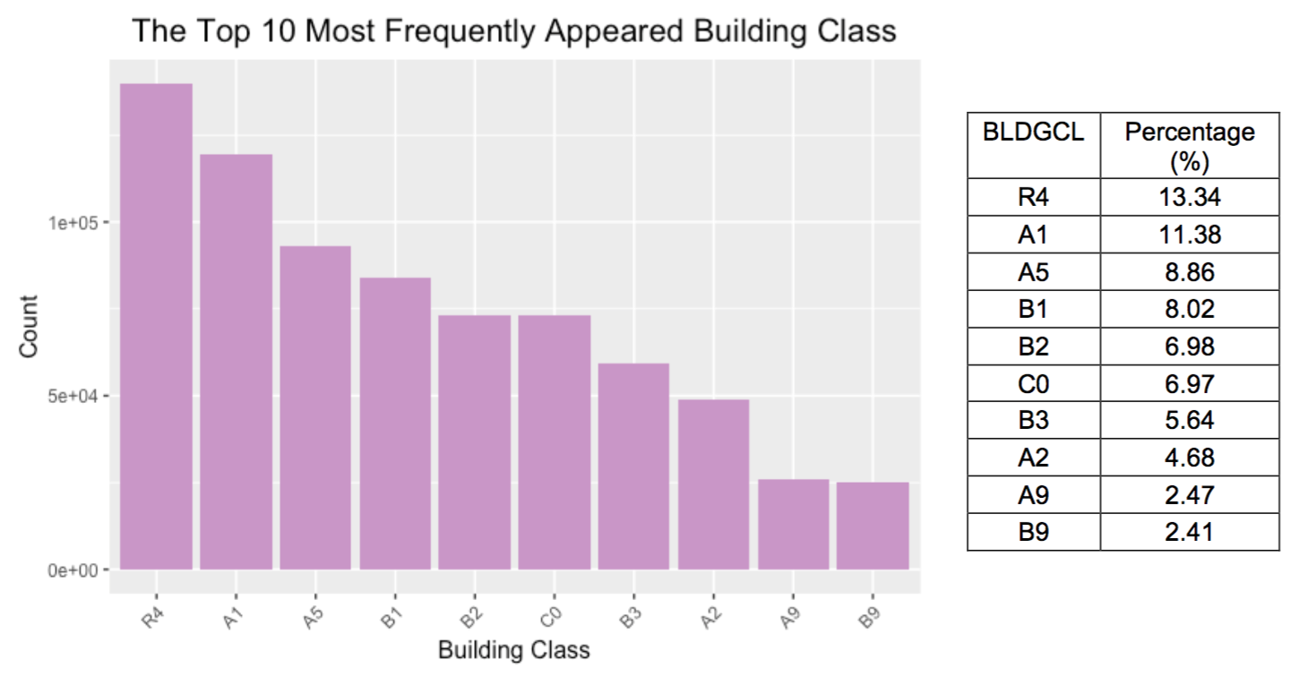
The graphical EDA of some generic variables are listed below.
- BLDGCL: a nominal categorical variable that represents the building class
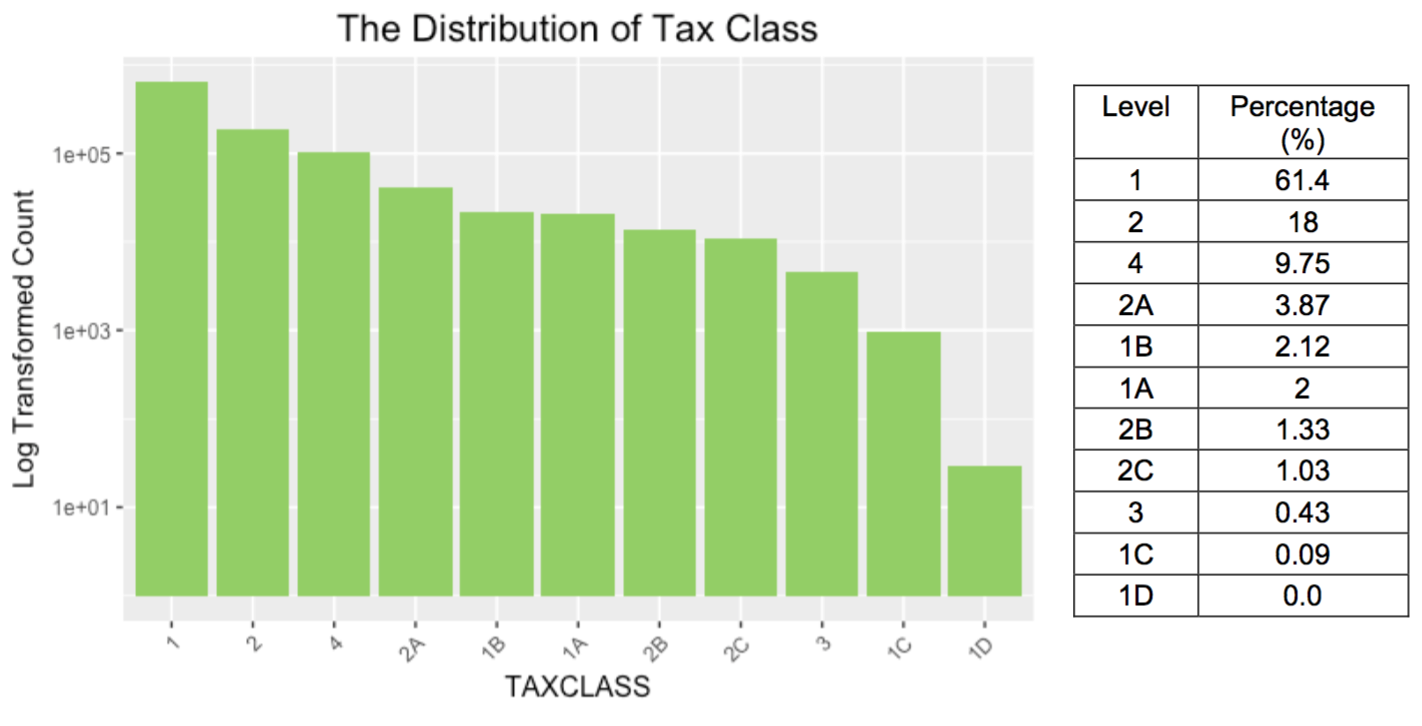
- TAXCLASS: a categorical variable that indicates the tax class of the property
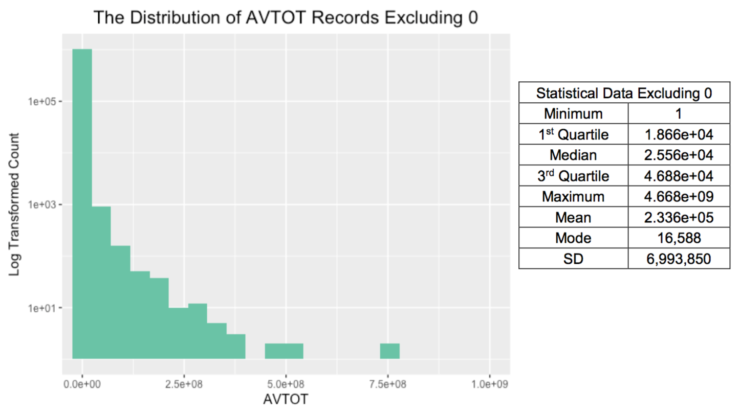
- AVTOT: a numerical variable which represents the assessed total value of the property
Data Cleaning
The data set is first cleaned by removing less informative and poorly populated variables and by filling in the missing values. Then, 13 most representative and well populated variables are selected, based on which 48 expert variables are created.
The data cleaning process includes:
- Removing variables
Less informative variables and poorly populated variables) were removed. - Filling missing values
Missing values are filled by a few different methods in a certain order. Firstly, the missing value is replaced by the average value of the fields grouped by ZIP. If it is not available, the average value of the fields grouped by ZIP3 is used, and then that of the fields grouped by BORO (Borough Code). - Adjusting and combining existing variables
Some variables were created for a more meaningful representation
Feature Engineering
We created features (variables) that make machine learning algorithms work by using domain knowledge of the data. Below is a summary of the 61 variables used in the models grouped into six columns.
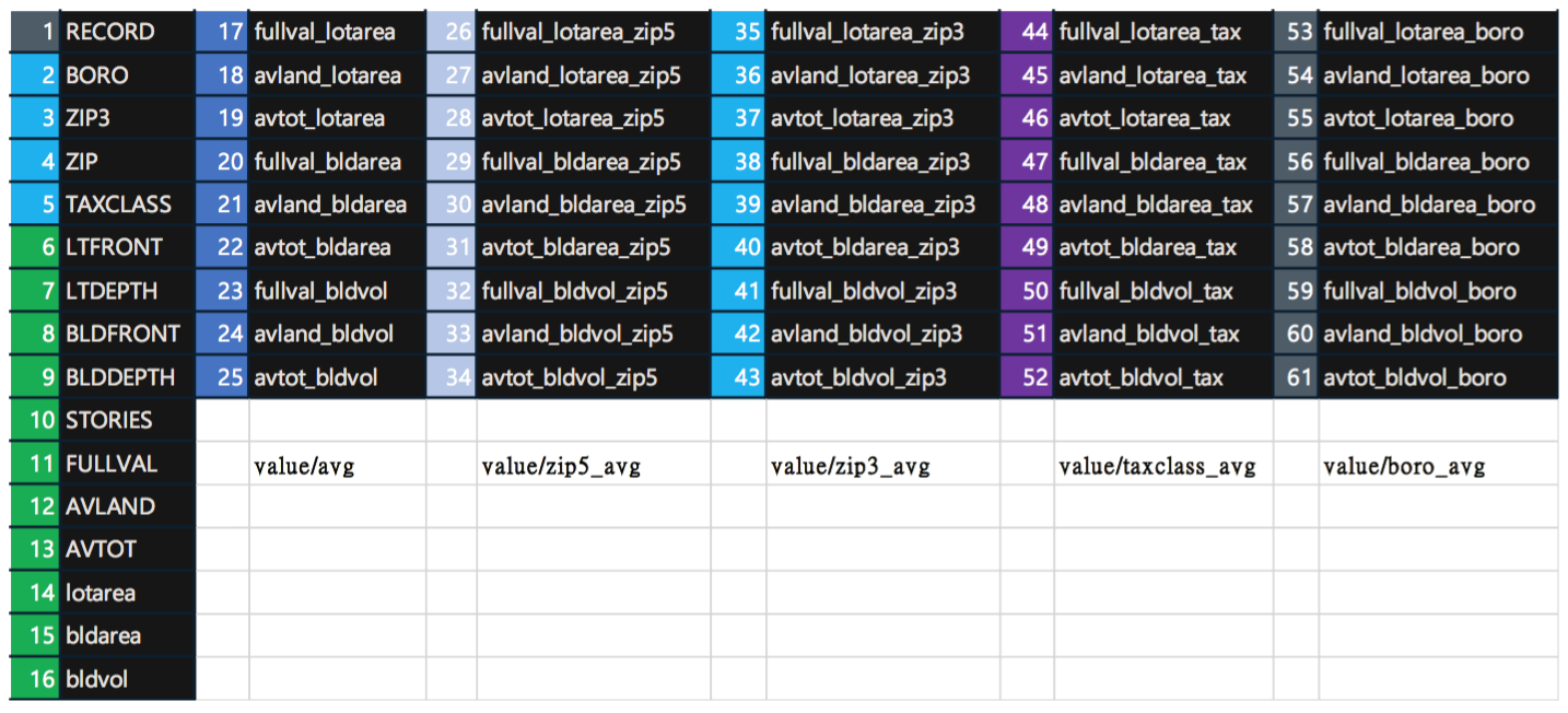
- Basic variables – column 1
The most useful and meaningful variables selected from the original data set, along with the three basic variables created out of the original variables - Baseline ratio variables – column 2
These variables are created by dividing value variables by area/volume variables to get the per area/volume number of the record - Grouping variables – column 3-6
The baseline ratio variables are then grouped by ZIP5, ZIP3, TAXCLASS and BORO, giving a comparison of the variables based on the average value of these variables in each group.
Snippet codes of feature engineering
ny_set=ny_set%>%
  group_by(BORO)%>%
  mutate(fullval_lotarea_boro=fullval_lotarea/mean(fullval_lotarea),
         avland_lotarea_boro=avland_lotarea/mean(avland_lotarea),
         avtot_lotarea_boro=avtot_lotarea/mean(avtot_lotarea),
         fullval_bldarea_boro=fullval_bldarea/mean(fullval_bldarea),
         avland_bldarea_boro=avland_bldarea/mean(avland_bldarea),
         avtot_bldarea_boro=avtot_bldarea/mean(avtot_bldarea),
         fullval_bldvol_boro=fullval_bldvol/mean(fullval_bldvol),
         avland_bldvol_boro=avland_bldvol/mean(avland_bldvol),
         avtot_bldvol_boro=avtot_bldvol/mean(avtot_bldvol))
Algorithms
A few algorithms are used to build unsupervised models from the data set, and the then the scores are weighted to get a final fraud score for each record.
A. Heuristic Approach
-
Z-scaling
The first process used on our data set is Z-scaling. Z-scaling is done to normalize all the numeric variables. For every value in a column, the mean of that column is subtracted from the value and divided by the standard deviation of the column. Z-scaling is extremely beneficial because it ensures that all input variables have the same treatment in the model and the coefficients of the model are not scaled with respect to the units of the inputs. Also, this makes it easier to interpret the results. -
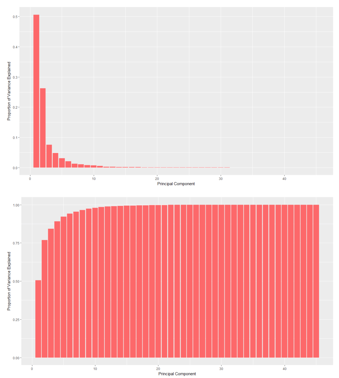
Principal Component Analysis (PCA)
PCA is a statistical procedure that uses an orthogonal transformation to convert a set of observations of possibly correlated variables called principal components. This transformation is defined in a way that the first possible principal component has the largest possible variance (that is, it accounts for the maximum variability in the data as possible). The resulting vectors are an uncorrelated orthogonal basis set.
The purpose of using PCA is to reduce the dimensionality of the data. PCA was run on the data set and only the variables that account for majority of the variance are selected. A built-in package in R is used to run PCA. Post running the PCA on the data, the outputs are z-scaled again, and PCA z-score is computed.
- Mahalanobis Distance
The fraud score (S) is calculated using z-scaling then Euclidean (Mahalanobis Distance). Where n = 2 (Euclidean)
Snippet codes of heuristic methods
ny_scale=data.frame(scale(ny_set[,17:61]))
ny.pca =prcomp(ny_scale)
pr.var =ny.pca$sdev ^2
eig=pr.var/sum(pr.var)
pve1=data.frame(eig)

ny_pca_out=data.frame(ny.pca$x)
ny_pca_scale=data.frame(scale(ny_pca_out[,1:8]))
loading=data.frame(ny.pca$rotation)
f <- function(x,n) abs(x)^(n)
ny_pca_scale$z_pca=(rowSums(apply(ny_pca_scale[,1:8],2,f,n=2)))^(1/2)
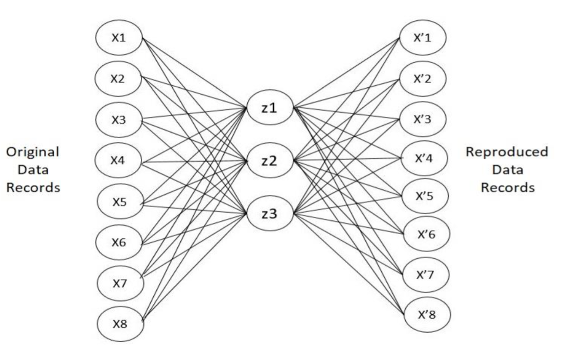
B. Neural Network
- Autoencoder The autoencoder is a neural network. The autoencoder can be trained on a training dataset from which it can learn the relationship between the data. H2O package is used to run Autoencoder. Functionally, autoencoder is trained and then used to reconstruct the original record. This is essentially using its results from training to reconstruct the original data. The error of reconstruction is the fraud score since it corresponds to the anomalous behavior of that data record.
- Mahalanobis Distance
Same as the heuristic method, we used Mahalanobis distance to list the fraud score.
Snippet codes of Neural Net and Mahalanobis Distance
ny_auto=autoencoder(ny_pca_scale[,1:8], hiddenLayers = c(3), batchSize = 30000,
            learnRate = 1e-5, momentum = 0.5, L1 = 1e-3, L2 = 1e-3,
            robErrorCov = TRUE)

plot(ny_auto)
rX <- reconstruct(ny_auto,ny_pca_scale[,1:8])
ny_auto_z=data.frame(rX$reconstruction_errors)
ny_auto_z$z_auto=(rowSums(apply(ny_auto_z[,1:8],2,f,n=2)))^(1/2)
Combining The Fraud scores
Scores are combined through the method of quantile binning. The idea of quantile binning is that a variable or score is transformed into its quantile ranking. This method is used when we want to scale the outputs from several models, so we can combine them. The methodology is as follows:
- Bin the data into bins of equal population but unequal width
- Replace the original values (variable or score) with the bin number
- All the variables/scores are on equal scales
A weight of 50% is given to each model since there is no preference for a certain model. The formula used is stated below:
Score(final) = (Score from heuristic algorithm * 0.5) + (Score from Autoencoder * 0.5)
Result and investigation
Below is the fraud score distribution and the Cumulative Distribution Function (CDF) of fraud score generated by heuristic method and neural network.
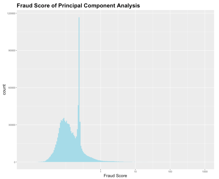
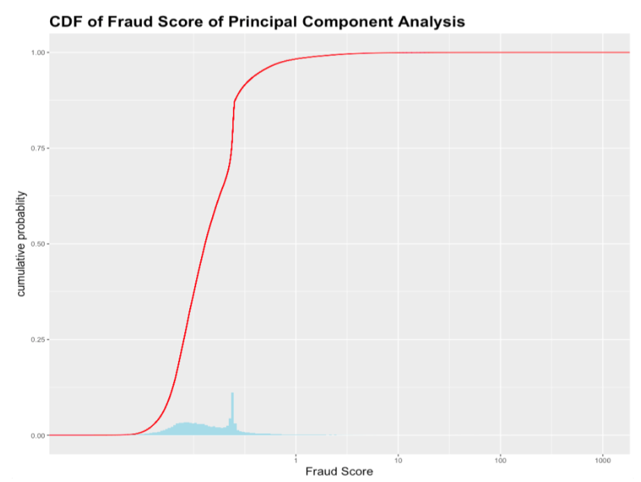
a. Heuristic Method
The graph is right skewed as expected. Most records have fraud score below 1 and a small portion of records have extremely high fraud score. More precisely, it can be seen from the CDF graph above that around 99% of the properties have fraud scores between 0 and 1, and 1% of the properties have a wide range of fraud score from 1 to extreme scores that are higher than1000.
Snippet code to calculate Fraud Score and CDF
ggplot(ny_auto_z,aes(x=z_auto))+
  geom_histogram(bins=200,fill="lightblue")+
  scale_x_log10(breaks=c(0,1,10,100,1000))

ggplot(ny_auto_z,aes(x=z_auto)) +
  stat_ecdf(color="red") +
  geom_histogram(bins=200,aes(y = (..count..)/sum(..count..)),fill="lightblue")+
  scale_x_log10(breaks=c(0,1,10,100,1000))
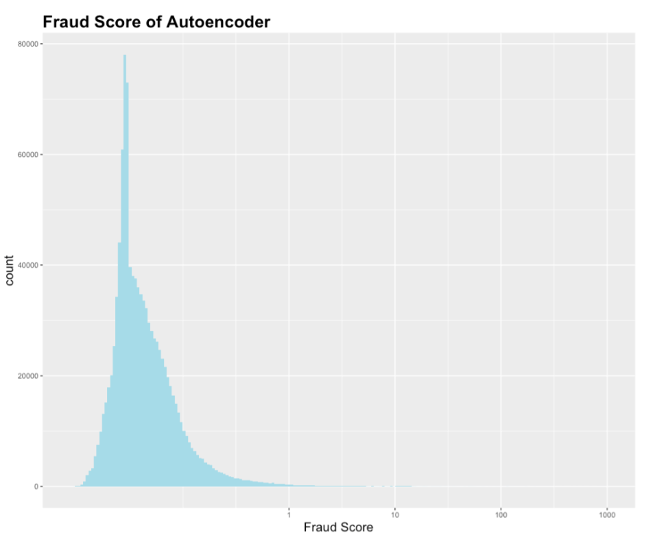
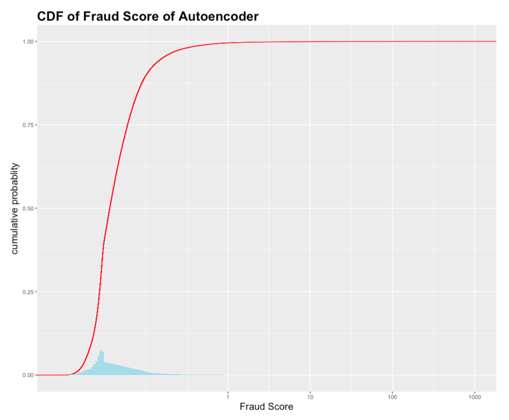
b. Neural network (Autoencoder)
The result of Autoencoder is like that of heuristic methods. The distribution of the fraud score generated by Autoencoder is also right skewed as expected. More precisely, in the CDF graph above, almost 99% of the properties have the fraud score between 0 and 1. The rest 1% of the properties have a fraud score widely spread in the range of 1 to 1000.
A further study was conducted on the top 1% high score records generated by the combined score of principal component analysis and autoencoder.
Conclusions
The top fraud properties found out have share certain patterns:
-
Some properties have unreasonably small lot/building front and lot/building depth. They are not missing values, thus not replaced by average value. Since the values are extremely small, such as 1, even if the full values are around average, the ratios will be very high compared to the average. Thus, these properties pop up as top fraud properties.
-
Some properties have extremely high full values, assessed land values and assessed total values. Since these values are extremely high, such as $10 billion, even if the lot/building front and lot/building depth values are around average, the ratios will be very high compared to the peer average. Thus, these properties pop up as top fraud properties.