
Improving Student Recruitment in USC Suzanne Dworak-Perk, School of Social Work
Photo by Social Work USC
Programming Language: Python
I will briefly explain the business problem and recommendations, followed by how to build several predictive models to get actionable recommendations.
Summary
- Business Problem: 45% of students who accepted offer didn’t end up joining
- Recommendations: Tame influential factors and Sell diversity more
Business Problem
- Students not joining school after accepting the offers
- Waitlist candidates denied the chance to fill up vacant seats
- Need for a data based approach
Recommendations
- Do regular surveys to understand student pain points regarding choice of university
- Ensure shorter turnaround time for applications by increasing number of reviewers
- Nominate students ambassadors from eclectic backgrounds and ask them to share their stories with new admits
Note: Performed data cleaning and feature engineering before building models. Codes below focusing more on building predictive models using Logistic Regression, Decision Tree, Boosted Tree and Random Forest
Preliminary
import pandas as pd
import numpy as np
import matplotlib.pyplot as plt
data = pd.read_csv("data_master2.csv")
data.head()
| Gap | Reaction Time | undergraduate gpa | Exp avg | Sop avg | GPA avg | LoR avg | distance to campus | length | Response-letter sent | ... | dposit received | follow up | 1411 | 272 | 1632 | 1645 | master or not | 1st gen | residency | response | |
|---|---|---|---|---|---|---|---|---|---|---|---|---|---|---|---|---|---|---|---|---|---|
| 0 | 0.000000 | 1.281658 | 0.000000 | 0.789351 | 0.967457 | 1.047935 | 1.210126 | 0.042364 | 0.920615 | 0.681886 | ... | 0 | 0 | 0 | 0 | 0 | 0 | 0 | 0 | 1 | 0 |
| 1 | 1.160673 | 1.222046 | 0.000000 | 1.262962 | 0.846525 | 1.047935 | 0.672292 | 0.037201 | 0.920615 | 0.762108 | ... | 1 | 0 | 0 | 0 | 0 | 0 | 0 | 0 | 1 | 1 |
| 2 | 0.000000 | 0.238448 | 0.402624 | 0.000000 | 0.000000 | 0.000000 | 0.000000 | 0.084369 | 0.920615 | 0.681886 | ... | 1 | 0 | 0 | 0 | 0 | 0 | 0 | 0 | 1 | 0 |
| 3 | 16.997967 | 2.503705 | 0.680190 | 1.578703 | 0.725593 | 0.261984 | 0.806751 | 0.033190 | 1.380922 | 0.200555 | ... | 1 | 0 | 0 | 0 | 0 | 0 | 0 | 0 | 1 | 1 |
| 4 | 0.875911 | 0.923986 | 0.686290 | 1.105092 | 0.967457 | 0.261984 | 0.806751 | 0.793829 | 1.380922 | 0.000000 | ... | 1 | 0 | 1 | 0 | 0 | 0 | 0 | 0 | 1 | 1 |
5 rows × 29 columns
data.info()
<class 'pandas.core.frame.DataFrame'>
RangeIndex: 5091 entries, 0 to 5090
Data columns (total 29 columns):
Gap                     5091 non-null float64
Reaction Time           5091 non-null float64
undergraduate gpa       5091 non-null float64
Exp avg                 5091 non-null float64
Sop avg                 5091 non-null float64
GPA avg                 5091 non-null float64
LoR avg                 5091 non-null float64
distance to campus      5091 non-null float64
length                  5091 non-null float64
Response-letter sent    5091 non-null float64
last 60/90 gpa          5091 non-null float64
decision 1              5091 non-null int64
decision 2              5091 non-null int64
academic con            5091 non-null int64
campus1                 5091 non-null int64
campus2                 5091 non-null int64
campus3                 5091 non-null int64
campus4                 5091 non-null int64
campus5                 5091 non-null int64
dposit received         5091 non-null int64
follow up               5091 non-null int64
1411                    5091 non-null int64
272                     5091 non-null int64
1632                    5091 non-null int64
1645                    5091 non-null int64
master or not           5091 non-null int64
1st gen                 5091 non-null int64
residency               5091 non-null int64
response                5091 non-null int64
dtypes: float64(11), int64(18)
memory usage: 1.1 MB
data.describe()
| Gap | Reaction Time | undergraduate gpa | Exp avg | Sop avg | GPA avg | LoR avg | distance to campus | length | Response-letter sent | ... | dposit received | follow up | 1411 | 272 | 1632 | 1645 | master or not | 1st gen | residency | response | |
|---|---|---|---|---|---|---|---|---|---|---|---|---|---|---|---|---|---|---|---|---|---|
| count | 5091.000000 | 5091.000000 | 5091.000000 | 5091.000000 | 5091.000000 | 5091.000000 | 5091.000000 | 5091.000000 | 5091.000000 | 5091.000000 | ... | 5091.000000 | 5091.000000 | 5091.000000 | 5091.000000 | 5091.0 | 5091.000000 | 5091.000000 | 5091.000000 | 5091.000000 | 5091.000000 |
| mean | 1.000000 | 1.000000 | 1.000000 | 1.000000 | 1.000000 | 1.000000 | 1.000000 | 1.000000 | 1.000000 | 1.000000 | ... | 0.694166 | 0.000589 | 0.029464 | 0.001768 | 0.0 | 0.000982 | 0.029071 | 0.510509 | 0.622864 | 0.592025 |
| std | 6.258178 | 0.678768 | 0.114475 | 0.357235 | 0.253189 | 0.290475 | 0.267889 | 1.873968 | 0.203576 | 1.454722 | ... | 0.460805 | 0.024270 | 0.169119 | 0.042012 | 0.0 | 0.031327 | 0.168022 | 0.499939 | 0.484717 | 0.491507 |
| min | 0.000000 | 0.000000 | 0.000000 | 0.000000 | 0.000000 | 0.000000 | 0.000000 | 0.000000 | 0.000000 | 0.000000 | ... | 0.000000 | 0.000000 | 0.000000 | 0.000000 | 0.0 | 0.000000 | 0.000000 | 0.000000 | 0.000000 | 0.000000 |
| 25% | 0.082905 | 0.596120 | 0.924204 | 0.631481 | 0.846525 | 0.785951 | 0.806751 | 0.025895 | 0.920615 | 0.200555 | ... | 0.000000 | 0.000000 | 0.000000 | 0.000000 | 0.0 | 0.000000 | 0.000000 | 0.000000 | 0.000000 | 0.000000 |
| 50% | 0.291970 | 0.894180 | 1.003509 | 0.947222 | 0.967457 | 1.047935 | 1.075668 | 0.066217 | 0.920615 | 0.481331 | ... | 1.000000 | 0.000000 | 0.000000 | 0.000000 | 0.0 | 0.000000 | 0.000000 | 1.000000 | 1.000000 | 1.000000 |
| 75% | 1.091585 | 1.192240 | 1.082814 | 1.262962 | 1.209321 | 1.309919 | 1.210126 | 0.762470 | 0.920615 | 1.082995 | ... | 1.000000 | 0.000000 | 0.000000 | 0.000000 | 0.0 | 0.000000 | 0.000000 | 1.000000 | 1.000000 | 1.000000 |
| max | 431.570789 | 7.838980 | 1.220072 | 1.578703 | 1.693050 | 1.309919 | 1.344584 | 18.911538 | 1.841230 | 18.410918 | ... | 1.000000 | 1.000000 | 1.000000 | 1.000000 | 0.0 | 1.000000 | 1.000000 | 1.000000 | 1.000000 | 1.000000 |
8 rows × 29 columns
X = data.loc[:,'Gap':'residency']
y = data.loc[:,'response']
Logistic Regression
from sklearn.linear_model import LogisticRegression
from sklearn.model_selection import train_test_split
logreg = LogisticRegression()
X_train, X_test, y_train, y_test = train_test_split(X, y, test_size=0.4, random_state=42)
print("Training features/target:", X_train.shape, y_train.shape)
print("Testing features/target:", X_test.shape, y_test.shape)
Training features/target: (3054, 28) (3054,)
Testing features/target: (2037, 28) (2037,)
logreg.fit(X_train, y_train)
logreg.score(X_train, y_train)
0.94368041912246237
y_pred = logreg.predict(X_test)
from sklearn.metrics import roc_curve
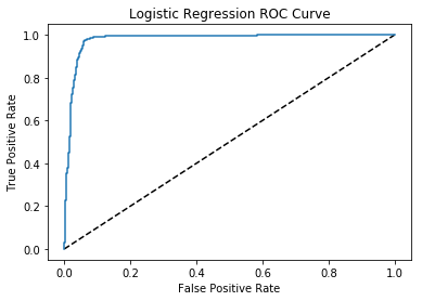
y_pred_prob = logreg.predict_proba(X_test)[:,1]
fpr, tpr, thresholds = roc_curve(y_test, y_pred_prob)
plt.plot([0, 1], [0, 1], 'k--')
plt.plot(fpr, tpr, label='Logistic Regression')
plt.xlabel('False Positive Rate')
plt.ylabel('True Positive Rate')
plt.title('Logistic Regression ROC Curve')
plt.show()
from sklearn.metrics import confusion_matrix
confusion_matrix(y_test, y_pred)
array([[ 772,   77],
       [  12, 1176]])
pd.crosstab(y_test, y_pred, rownames=['True'], colnames=['Predicted'], margins=True)
| Predicted | 0 | 1 | All |
|---|---|---|---|
| True | |||
| 0 | 772 | 77 | 849 |
| 1 | 12 | 1176 | 1188 |
| All | 784 | 1253 | 2037 |
Random Forest
from sklearn.ensemble import RandomForestClassifier
rf = RandomForestClassifier(n_estimators=10, random_state=0)
rf.fit(X_train, y_train)
rf.score(X_test, y_test)
0.95778105056455576
y_pred2 = rf.predict(X_test)
pd.crosstab(y_test, y_pred2, rownames=['True'], colnames=['Predicted'], margins=True)
| Predicted | 0 | 1 | All |
|---|---|---|---|
| True | |||
| 0 | 791 | 58 | 849 |
| 1 | 28 | 1160 | 1188 |
| All | 819 | 1218 | 2037 |
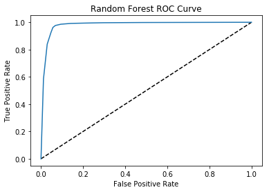
y_pred_prob2 = rf.predict_proba(X_test)[:,1]
fpr, tpr, thresholds = roc_curve(y_test, y_pred_prob2)
plt.plot([0, 1], [0, 1], 'k--')
plt.plot(fpr, tpr, label='Random Forest')
plt.xlabel('False Positive Rate')
plt.ylabel('True Positive Rate')
plt.title('Random Forest ROC Curve')
plt.show()
Decision Tree
from sklearn.tree import DecisionTreeClassifier
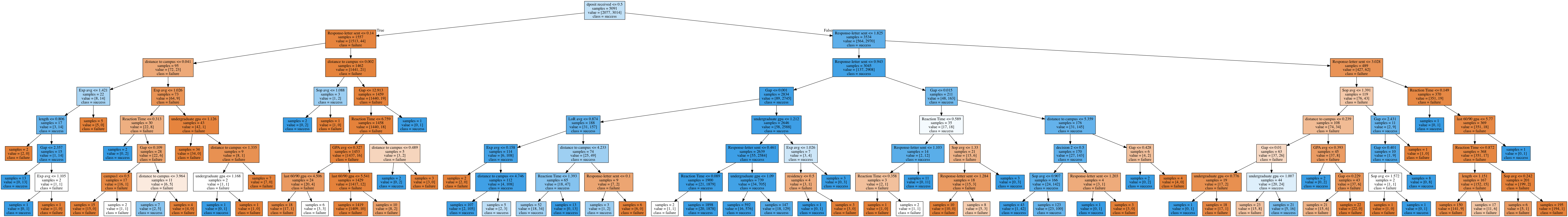
tree = DecisionTreeClassifier(max_depth=7, random_state=0)
tree.fit(X_train, y_train)
tree.score(X_test, y_test)
0.9464899361806578
y_pred3 = tree.predict(X_test)
pd.crosstab(y_test, y_pred3, rownames=['True'], colnames=['Predicted'], margins=True)
| Predicted | 0 | 1 | All |
|---|---|---|---|
| True | |||
| 0 | 762 | 87 | 849 |
| 1 | 22 | 1166 | 1188 |
| All | 784 | 1253 | 2037 |
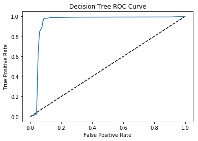
y_pred_prob3 = tree.predict_proba(X_test)[:,1]
fpr, tpr, thresholds = roc_curve(y_test, y_pred_prob3)
plt.plot([0, 1], [0, 1], 'k--')
plt.plot(fpr, tpr, label='Decision Tree')
plt.xlabel('False Positive Rate')
plt.ylabel('True Positive Rate')
plt.title('Decision Tree ROC Curve')
plt.show()
Boosted Tree
from sklearn.ensemble import AdaBoostClassifier
boost = AdaBoostClassifier()
boost.fit(X_train, y_train)
boost.score(X_test, y_test)
0.95041728031418748
y_pred4 = boost.predict(X_test)
pd.crosstab(y_test, y_pred4, rownames=['True'], colnames=['Predicted'], margins=True)
| Predicted | 0 | 1 | All |
|---|---|---|---|
| True | |||
| 0 | 778 | 71 | 849 |
| 1 | 30 | 1158 | 1188 |
| All | 808 | 1229 | 2037 |
y_pred_prob4 = boost.predict_proba(X_test)[:,1]
fpr, tpr, thresholds = roc_curve(y_test, y_pred_prob4)
plt.plot([0, 1], [0, 1], 'k--')
plt.plot(fpr, tpr, label='Boosted Tree')
plt.xlabel('False Positive Rate')
plt.ylabel('True Positive Rate')
plt.title('Boosted Tree ROC Curve')
plt.show()

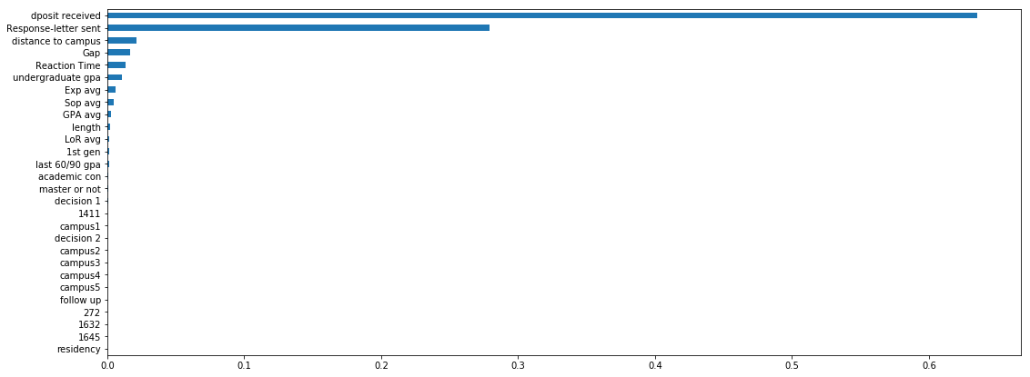
Feature Importances
%matplotlib inline
pd.Series(tree.feature_importances_, index=X.columns).sort_values(0, ascending=True).plot.barh(figsize=(18,7));
from sklearn.tree import export_graphviz
import sys, subprocess
from IPython.display import Image

export_graphviz(tree, feature_names=X.columns, class_names=['failure','success'],
                out_file='ml-good.dot', impurity=False, filled=True)
subprocess.check_call([sys.prefix+'/bin/dot','-Tpng','ml-good.dot',
                       '-o','ml-good.png'])
Image('ml-good.png')