Supervised Model for Detecting Fraudulent Transactions

photo byTNW
Programming Language: R and SQL

Project Objective

Our Goal is to build a prediction model for detecting fraudulent transactions in applications data based on historical data, in real time. To achieve this objective, we have used several machine learning models to predict the records that are fraudulent.

Data Description

The applications dataset contains a total of 94,866 records and 10 fields. Out of these variables, 2 are date variables, 3 are string variables, and 5 are categorical variables. All the fields are 100% populated. Below is a table of the summary of the data, and a more detailed description of each field follows.

Statistical Summary

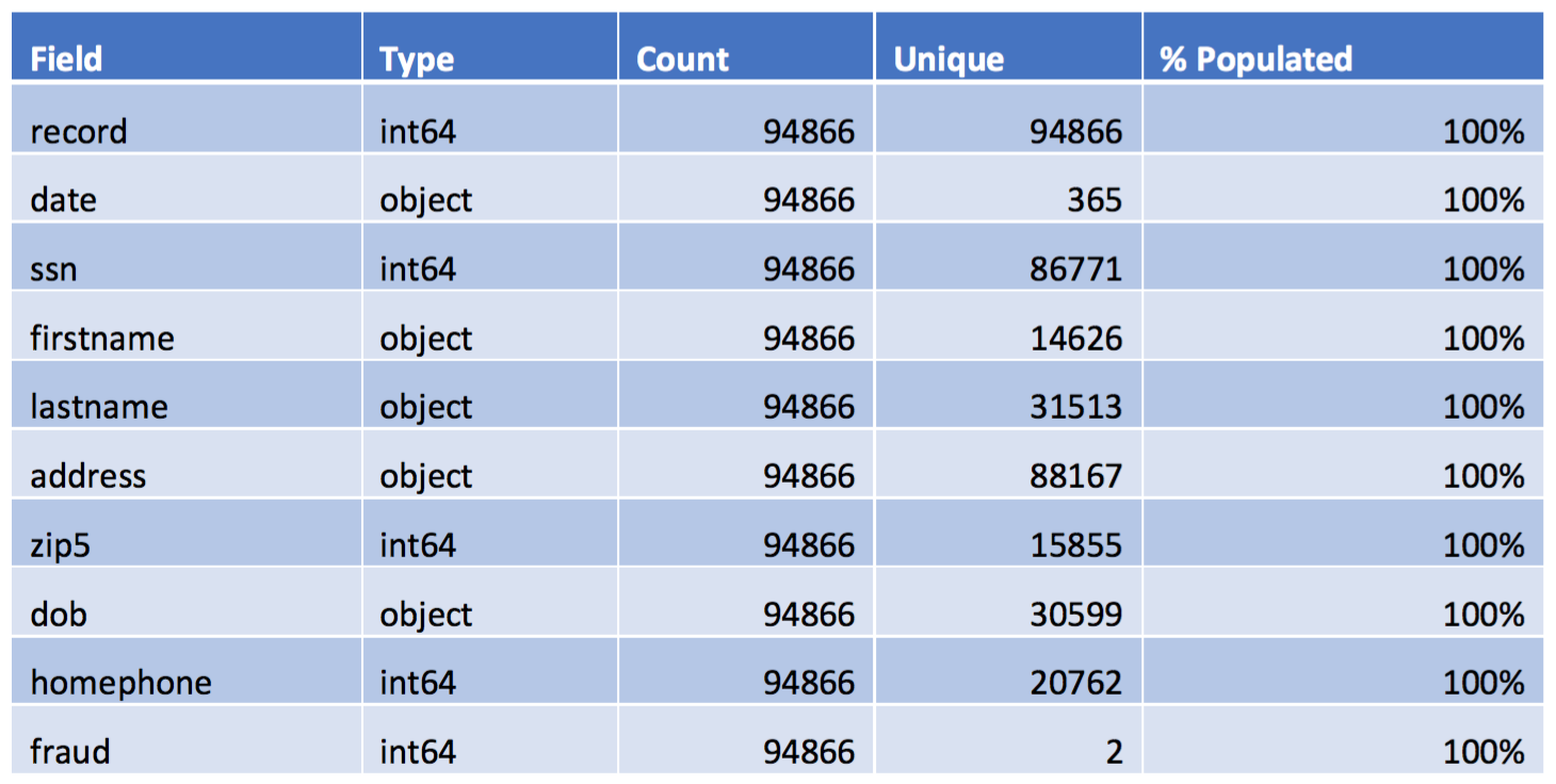
• record: the ordinal reference number for each product application record
• date: Social Security Number
• firstname: the first name of each applicant
• lastname: the last name of each applicant
• address: the address of each applicant
• zip5: the zip code of each applicant
• dob: the date of birth of each applicant
• homephone: the phone number of each applicant
• fraud: whether application

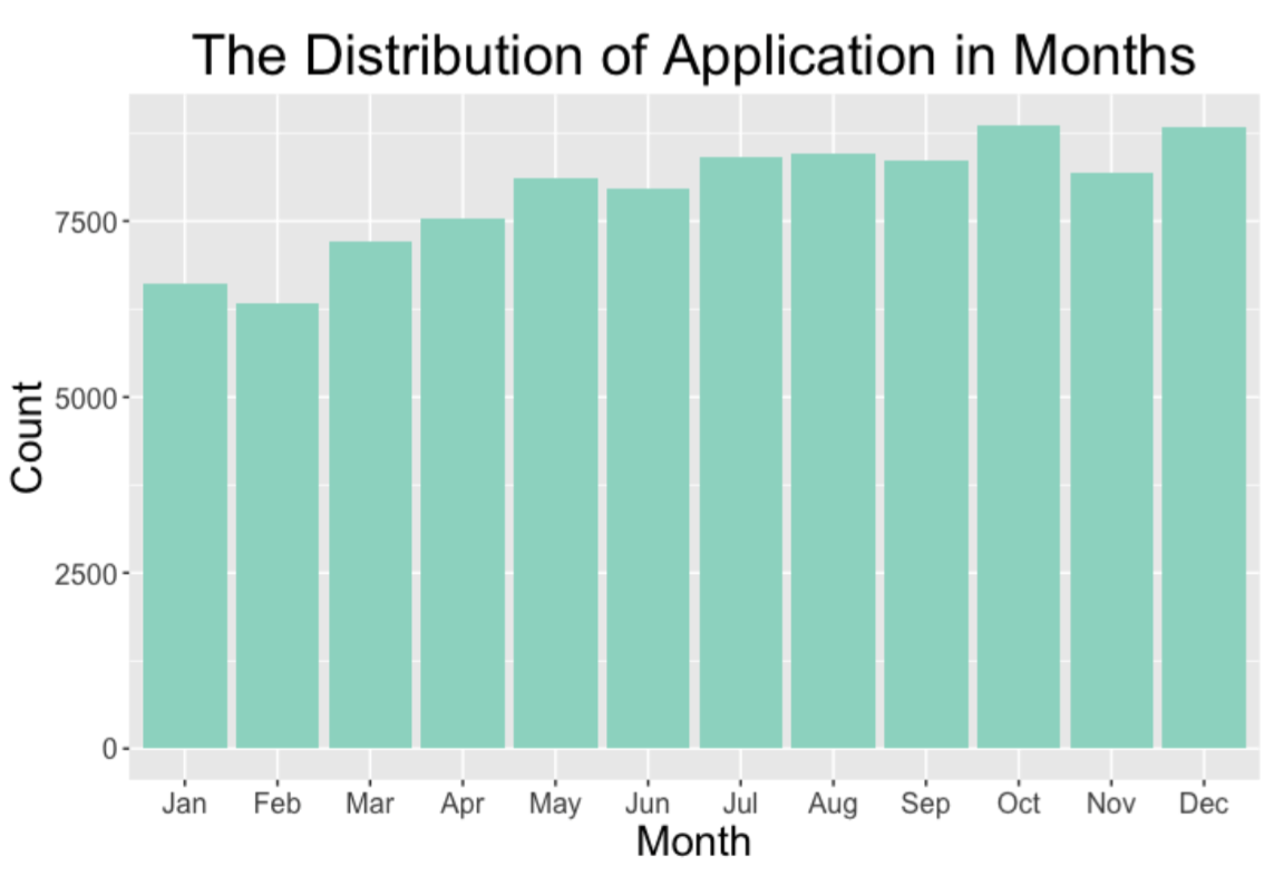
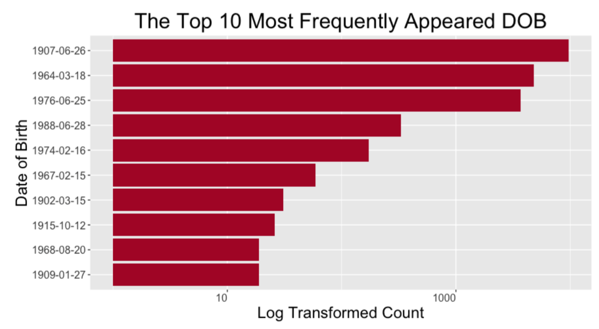
Descriptive analyses of some variables are listed below.

Data Cleaning

The only issues that call for attention are frivolous values and records with omitted zeros at the start.

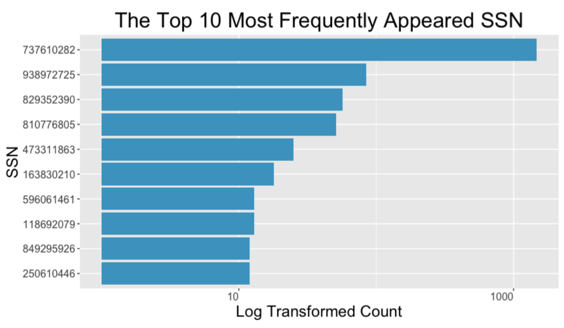
1. Based on the distribution of the SSN field, we noticed that there is one SSN number, 737610282, that has a substantially large count, i.e., 1478. Also, This SSN has a count more than 10 times the count of other SSNs. Thus, we believe this is a frivolous value. We address this issue when building expert variables using the SSN.

2. Based on the distribution of the home phone field, we noticed that there is one phone number, 9105580920, that has a substantially large count, i.e., 4974. Also, this home phone number has a count more than 10 times the count of other home phone numbers. Thus, we believe this is a frivolous value. We address this issue when building expert variables using the home phone.

3. For the zip code column, we found that some of the zip codes have less than five digits. This is because the file automatically omits the leading zeros. Therefore, we add leading zeros to these zip codes to make them consistent with other zip codes.

Feature Engineering

From the 10 variables that we have in the original dataset, we created four types of variables. Each type of variable corresponds to a time window.

Time Window We assume that record numbers are assigned in a time ascending order. The application with record number 1 was the first application received on Jan 1st, 2016. If two applications were received on the same day, then the one received earlier would have a smaller record number.

• 3-day time window
• 15-day time window
• 30-day time window
• 60-day time window

a. Type I Variables

Type I variables summarize the count of records associated with specific values in one entity or combinations of entities, such as SSN, name with date of birth, address, home phone, name with address and name with zip code, in a time window. For example:

• ssn_1_ss: number of records with same SSN in 3-day time window.
• ndob_1_ss: number of records with same name and date of birth in 3-day time window.
• address_1_ss: number of records with same address in 3-day time window.
• phone_1_ss: number of records with same home phone number in 3-day time window.
• nadd_1_ss: number of records with same name and address in 3-day time window.
• nzip_1_ss: number of records with same name and zip code in 3-day time window.

In an analogous way, we built type I variables for the 15-day, 30-day and 60- day time windows. Thus, we built (6*4 = 24) type I variables in total.

b. Type II Variables

Type II variables summarize the count of records associated with specific values in one entity or combinations of entities like SSN, name with date of birth, address, home phone, name with address, name with zip code associated with specific values in another entity or combination of entities such as address, name with date of birth, name with zip code and home phone number, in a particular time window.

c. Type III Variables

Type III variables summarize the counts of frauds associated with specific values in one entity or combination of entities such as SSN, name with date of birth, address, home phone number, name with address and name with zip code, in a particular time window.

d. Type IV Variables

Type IV variables show how many days ago, specific values in one entity or combinations of entities were last seen. For example, if the entity was last seen today, then the value equals to 0. If the entity was last seen yesterday, the value equals to 1. If the entity is seen for the first time, the value equals to 366.

Snippet of the code We used SQL in R to create those expert variables, another method is using data.table

nadd= dbGetQuery(con,
                 "SELECT a.record,
                 COUNT(CASE WHEN a.date_date - b.date_date BETWEEN 0 AND 59 THEN b.record ELSE NULL END)-1  AS nadd_1_w,
                 COUNT(CASE WHEN a.date_date - b.date_date BETWEEN 0 AND 29 THEN b.record ELSE NULL END)-1  AS nadd_1_m,
                 COUNT(CASE WHEN a.date_date - b.date_date BETWEEN 0 AND 14 THEN b.record ELSE NULL END)-1  AS nadd_1_s,
                 COUNT(CASE WHEN a.date_date - b.date_date BETWEEN 0 AND 2 THEN b.record ELSE NULL END)-1  AS nadd_1_ss,
                 COUNT(DISTINCT CASE WHEN a.date_date - b.date_date BETWEEN 0 AND 59 THEN b.homephone ELSE NULL END)-1 AS nadd_phone_w,
                 COUNT(DISTINCT CASE WHEN a.date_date - b.date_date BETWEEN 0 AND 29 THEN b.homephone ELSE NULL END)-1 AS nadd_phone_m,
                 COUNT(DISTINCT CASE WHEN a.date_date - b.date_date BETWEEN 0 AND 14 THEN b.homephone ELSE NULL END)-1 AS nadd_phone_s,
                 COUNT(DISTINCT CASE WHEN a.date_date - b.date_date BETWEEN 0 AND 2 THEN b.homephone ELSE NULL END)-1  AS nadd_phone_ss,
                 sum(CASE WHEN a.date_date - b.date_date BETWEEN 0 AND 59 THEN b.fraud ELSE 0 END)-a.fraud AS nadd_fraud_w,
                 sum(CASE WHEN a.date_date - b.date_date BETWEEN 0 AND 29 THEN b.fraud ELSE 0 END)-a.fraud AS nadd_fraud_m,
                 sum(CASE WHEN a.date_date - b.date_date BETWEEN 0 AND 14 THEN b.fraud ELSE 0 END)-a.fraud AS nadd_fraud_s,
                 sum(CASE WHEN a.date_date - b.date_date BETWEEN 0 AND 2 THEN b.fraud ELSE 0 END)-a.fraud  AS nadd_fraud_ss                  
                 FROM data a, data b
                 WHERE a.date_date - b.date_date BETWEEN 0 AND 59
                 AND a.nadd = b.nadd
                 AND a.record>=b.record
                 GROUP BY 1")
nadd=nadd[,-1]

Feature Selection

The purpose of feature selection is to simplify our models for easier interpretation.Also, reducing the number of variables can reduce the training time. We created a total of 112 expert variables. However, before building models, we need to reduce the dimensionality of our data. In other words, we should reduce the number of variables and select useful ones using the process called feature selection.

a. Remove highly correlated expert variables

Since our expert variables are built associated with six original variables (ssn/homephone/address/ndob/nadd/nzip) and four time-windows, there is a great possibility of high correlation between variables. If a model includes too many highly correlated variables, it will make the estimation of coefficient in our linear regression unstable. We decided to remove one variable from each pair of variables that has a $|r_{x,y}| > 0.99$ and keep the others.

ss=train%>%select(ssn_1_w:address_day)
tmp <- cor(ss)
tmp[upper.tri(tmp)] <- 0
diag(tmp) <- 0
data.new <- ss[,!apply(tmp,2,function(x) any(abs(x) > 0.99))]

b. Kolmogorov-Smirnov(KS) - Top 30 Expert Variables

Kolmogorov-Smirnov is a nonparametric test to test for differences in the shape of two sample distributions and does not require data to follow a normal distribution. It is a nice, simple distribution independent measure of distance between two distributions – fraud and non-fraud groups. The farthest distance between whatever points in those two functions is the statistic of KS.

$$KS = max x \int_{xmin}^{x} [P_{fraud} - P_{non-fraud}] d_{x}$$

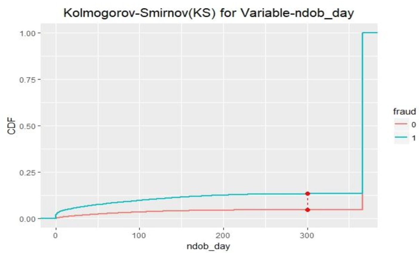
Above is the illustration of KS for variable ndob_day. Variable ndob_day has the largest KS among all expert variables, which indicates that this variable is the best indicator among all variables to predict fraud.

After implementing Kolmogorov-Smirnov(KS), we chose the top 30 variables that yield the highest KS. The following is a list of the 30 variables with their KS that we chose to use for building our models.

t=train%>%filter(response==1)
t1=train%>%filter(response==0)

names=names(data.new)
ks=data.frame()

for (j in names){
  kj=ks.test(t[,j],t1[,j],alternative="two.sided")
  ks[j,'KS']=kj[["statistic"]][["D"]]
}

ks$name=rownames(ks)
k=(ks%>%arrange(-KS))[1:30,]

c. Stepwise Selection

Stepwise selection method is a wrapper method. The process of stepwise selection is applied when building models. Wrapper method searches for an optimal feature tailored to a specific algorithm.

Forward Selection

In forward selection, it first builds n one-dimensional models, where n is the number of variables we have for our dataset. Then it chooses and selects the variable in which the model yields the lowest AIC (Akaike Information Criterion). Next, it builds n-1 two-dimensional models using the first variable it chose previously along with other variables. Then, it chooses the set of variables that the model yields the lowest AIC. The process continues until there is no more substantial model improvement.

After applying forward selection, we reduced our variables from 30 variables to 10 variables.

forward=step(glm.null,scope=list(lower=glm.null, upper=glm.full),direction ="forward",steps=5000)
summary(forward)
formula(forward)
glm.f=glm(formula(forward),data=train,family="binomial")

Backward Selection

Backward selection works in an opposite direction from forward selection. First, it builds a single model using all variables. Then, it builds n models by removing one variable each time and selects the best model which yields the lowest AIC. Again, it builds n-1 separate models by removing one variable each time and chooses the best model which yields the lowest AIC. The process continues until the model degradation is below an acceptable amount.

After applying backward selection, we reduced our variables from 30 variables to 16 variables.

back=step(glm.full)
summary(back)
formula(back)
glm.b=glm(formula(back),data=train,family="binomial")

We applied both selection methods when building our logistic regression model. The results are quite similar. Therefore, we decided to use forward selection (10 variables) since it has less variables than backward one. Since it is computationally expensive to do separate feature selections for each model, we also decided to use these 10 variables for different non-linear models.

The 10 variables are: ndob_day, ndob_1_ss, phone_fraud_w, ssn_fraud_w, nzip_1_w, ndob_fraud_w, ssn_day, phone_day, phone_fraud_s, and ssn_1_ss.

Building Models

In order to come up with the best possible model to identify the fraudulent applications, we tried multiple algorithms and then compared the performance of each algorithm on the out-of-time data. Before building models, we split our dataset into training, testing and validation. We used the last one month as validation and the remaining as traning-testing with ratio 7:3 respectively.

# 0 training, 1 test, 2 validation
data$val=ifelse(data$date_key>=306,"2","0")
set.seed(1)

# 30% testing
data[sample(1:77850,round(nrow(data[data$val==0,])*0.3)),'val']="1"   

table(data$val)
data$response=data$fraud
set=data%>%select(record,date_key,ssn_1_w:response)

a. Logistic Regression

Logistic regression is the most basic linear model in machine learning and is used when the output variable is categorical. Logistic regression can be seen as a special case of the generalized linear model (GLM) and thus analogous to linear regression. The key differences between these two models, first, the conditional distribution y|x is a Bernoulli distribution rather than a Gaussian distribution because the dependent variable is binary, and second, the predicted values are probabilities.

$$log(\frac{P_{1}}{P_{0}}) = \beta_{1}X_{1} + \beta_{2}X_{2} + ... + \beta_{p}X_{p}$$

train=set%>%filter(val=="0")
test=set%>%filter(val=="1")
val=set%>%filter(val=="2")
n <- k$name
f <- as.formula(paste("response ~", paste(n[!n %in% "response"], collapse = " + ")))
train$response=as.factor(train$response)
glm.null=glm(response~1, data=train,family="binomial")  ## no variable
glm.full=glm(f,data=train,family="binomial")            ## all variables : too many
contrasts(train$response)
summary(glm.full)

b. Boosted Trees

Boosting methods are very common and powerful algorithms. The algorithm for Boosting Trees evolved from the application of boosting methods to regression trees. The general idea is to compute a sequence of simple trees, where each successive tree is built for the prediction residuals of the preceding tree.

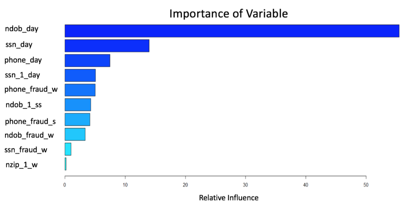
In our application of the algorithm, we used 10 expert variables generated from forward selection and 3000 number of trees. We also narrowed down the maximum number of splits to 4 because we do not want to over fit the model and we want our model to learn slowly the residual error from the previous trees. This means that the algorithm will build 3000 trees and each tree will have maximum 3*4+1=13 nodes.

Below graph shows the importance of variables in our boosted tree models. The higher relative influence of a variable means that variable plays a more important role in the model.

boost =gbm(formula(forward),data=train, distribution="bernoulli",n.trees =3000 , interaction.depth =4)

c. Neural Network

Neural Networks are a family of Machine Learning techniques and can extract hidden patterns within data. The neural net consists of the following components:

1. Input layer : the predictors that are fed as inputs to the neural net.
2. Hidden layer: a user defined layer with a specified number of neurons or nodes. The number of hidden layers determine the complexity of the neural network.
3. Output layer: the variable that we are trying to predict.

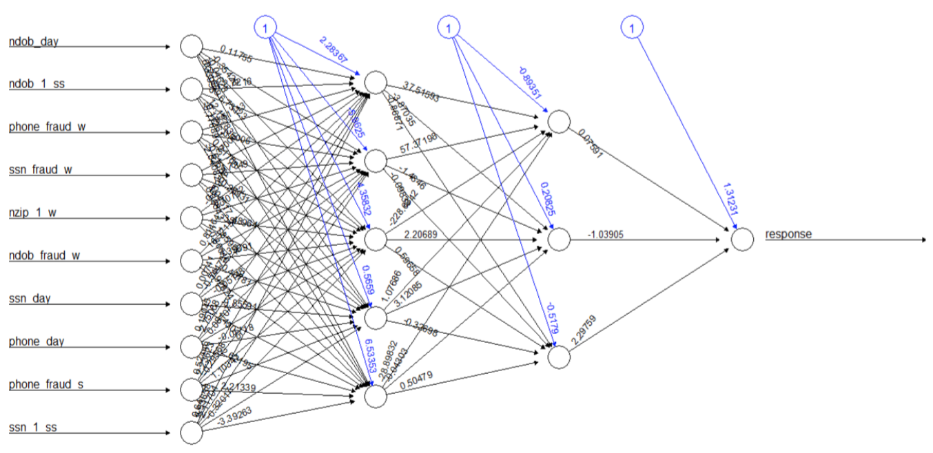
We used two hidden layers in our neural net model. The first layer has 5 nodes and the second layer has 3 nodes. For the algorithm in neural network, we used resilient back propagation and we used tanh as the activation function as shown in the formula below.

Below is the illustration of the neural network model we used.

nn <- neuralnet(formula(forward),data=train,hidden=c(5,3),algorithm = "rprop+", err.fct = "sse", act.fct  = "tanh", threshold =1,rep=1,linear.output=FALSE,lifesign ="full",stepmax=100000)

d. Support Vector Machine (SVM)

SVM is an algorithm for the classification of both linear and nonlinear data. It transforms the original data in a higher dimension, from where it can find a hyperplane for separation of the data using essential training tuples called support vectors. Since all we care about is distance, we can use a kernel to construct a distance measure in an abstract higher dimension. A kernel is a function that quantifies the similarity of two observations.

We used the e1071 library which contains implementations for a number of statistical learning methods including support vector machine. We used the svm() function to fit a support vector classifier and tune the hyper parameters such gamma, cost, and decision boundary (both linear and nonlinear). After several trials, we got the best FDRs by setting the decision boundary to non-linear (radial kernel), gamma to 1 and cost to 8.

train$response=as.factor(train$response)
n <- k$name
f <- as.formula(paste("response ~", paste(n[!n %in% "response"], collapse = " + ")))
sv=svm(formula(forward),data=train,kernel="radial",gamma=1,cost=8,probability=TRUE)

e. Random Forest

Random forest is a collection of many decision trees. When building these decision trees, each time a split in a tree is considered, a random sample of m predictors is chosen as split candidates from the full set of p predictors. The split is allowed to use only one of those m predictors.

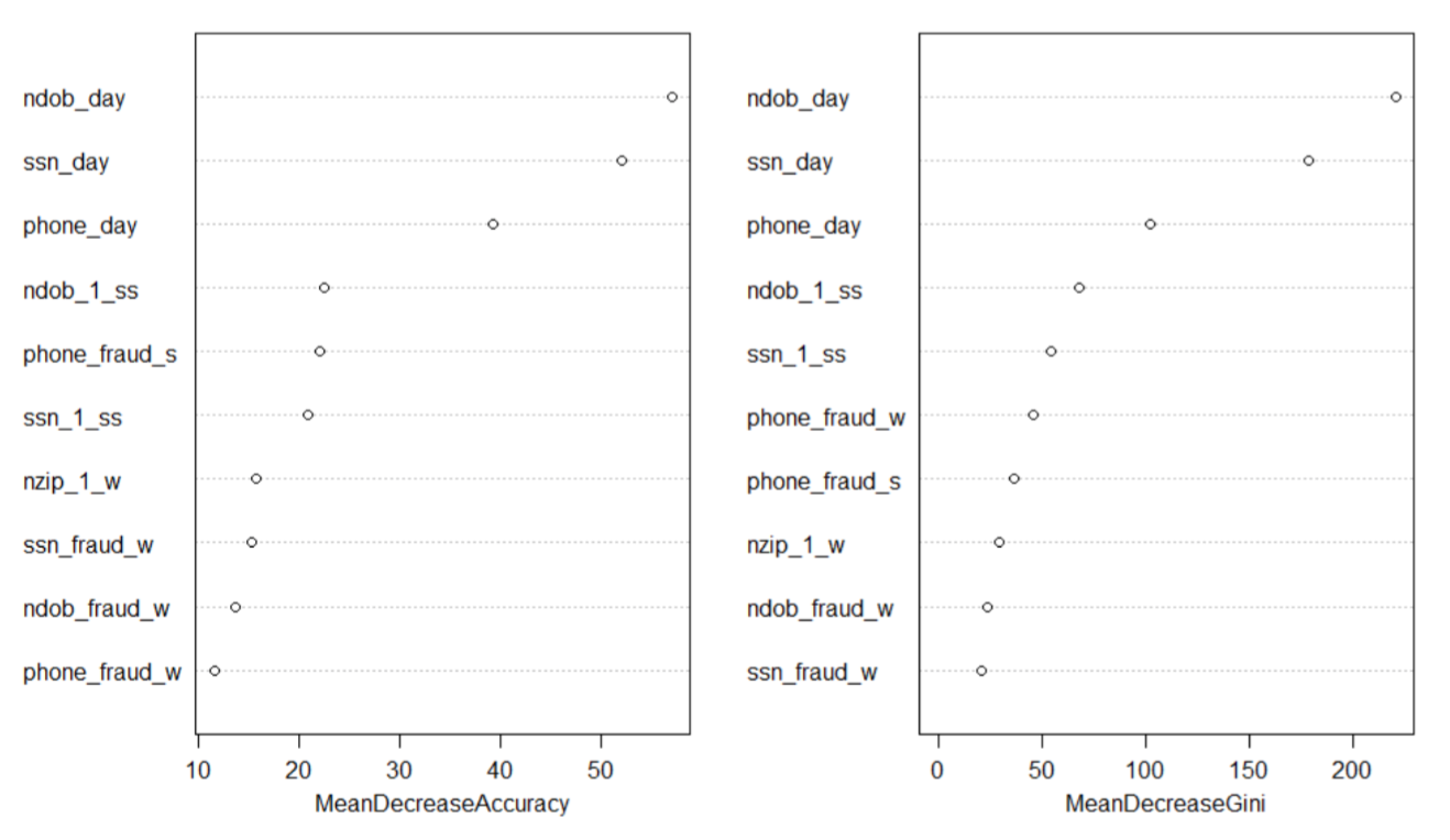
We used randomForest() function from randomForest library to build a random forest model with 1000 trees. We also set the number of variables randomly sampled as candidates at each split to 3 and the minimum size of terminal nodes to 50.

We used the mean decrease accuracy and the mean decrease Gini to rank order and determine which variables play important roles in our model. From the following graph we know ndob_day variable is the most significant variable in our model.

Mean Decrease Accuracy and Mean Decrease Gini

train$response=as.factor(train$response)
rf=randomForest(formula(forward),data=train,ntree=1000,mtry=3,nodesize=50,importance =TRUE)

Results

After we built our model, we ran five different models and summarized Fraud Detection Rate (FDR) for each model. Also, we created bin statistics and cumulative statistics for the number of good records, the number of bad records, Kolmogorov-Smirnov (KS) score, and false positive ratio. The high-level result of FDR at 10% population for each model is shown below.

FDR at 10% for each model

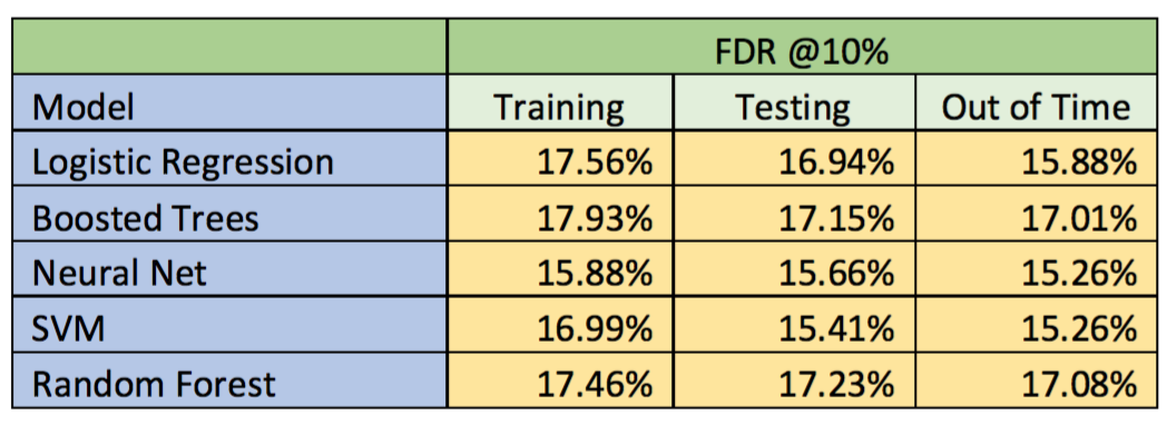
For all models, the FDR in training dataset is higher than the FDR in testing dataset. Also, the FDR in validation or out of time dataset is lower than both FDRs in training and testing dataset. Overall, the random forest model gives the highest FDR score in out of time dataset (17.08%) at 10% population.

Neural Net and SVM give somewhat lower scores of FDR at 10% population compared to Logistic Regression, Boosted Trees, and Random Forest because we think that we need to explore more on the hyper parameters such as gamma, cost, type of neural net algorithm to get better FDR scores. Also, we need to choose the best variables for non-linear models, because they do not fit in the model.

Conclusions

Based on the efficacy of the models, we conclude that random forest algorithm works the best on our dataset followed closely by boosted trees algorithm. The overall accuracy at 10% penetration is about 17%.

Reference

1. Introduction to Statistical Learning
2. Generalized Linear Model
3. Generalized Boosted Regression Models
4. SVM
5. Neural Net