

TalkingData AdTracking Fraud Detection
Photo by MIT
Programming Language: R
Problem Statement
TalkingData, China’s largest independent big data service platform, covers over 70% of active mobile devices nationwide. They handle 3 billion clicks per day, of which 90% are potentially fraudulent. Their current approach to prevent click fraud for app developers is to measure the journey of a user’s click across their portfolio, and flag IP addresses who produce lots of clicks, but never end up installing apps. With this information, they’ve built an IP blacklist and device blacklist.
While successful, they want to always be one step ahead of fraudsters. Therefore, the objective of this project is to build a predictive model that predicts whether a user will download an app after clicking a mobile app ad.
Description of The Data
Source: Kaggle.
The original dataset has 76 variables, among which there are seven original variables, two auxiliary variables, six categorical table variables and 61 expert variables. The variable called is_attributed is the dependent variable in the model we will build.
We build 61 expert variables on five-time windows which are 1 second, 3 seconds, 10 seconds, 30 seconds and 60 seconds. Before we do the feature selection to fit our model, we delete the first 60s records so that every record has a value for every expert variable.
Feature Engineering
From the descriptive analyses, most of the variables are categorical and are given in the format of IDs (app ID, device ID, etc.). Some types of the features we could build based on these categories are as below.
- Categorical tables: tables containing values directly associated with the dependent variable (i.e. the average of the dependent variable) for each possible category.
- Simple time-window counts: how many times this IP appeared in the last 60 seconds.
- Dynamic time-window counts: how many different devices associated with this
IP appeared in the last 60 seconds.
The term simple and dynamic for time-window are not formal terminologies.
a. Categorical tables
The common method to handle categorical variables is dummy encoding. What if some categorical variables contain too many levels, like zipcode? If we think we should keep this column in our model, then we might want to reduce the levels before we apply the dummy encoding; otherwise the feature dimension may explode. Another alternative to deal with too many levels is to build a categorical table, that is, to assign a value directly associated with the dependent variable (i.e. the average of the dependent variable) for each possible category. The pros of the categorical table encoding is that there is no dimensionality expansion as each categorical variable becomes one continuous variable, while the cons of doing so is the loss of interaction.
We can use sqldf or dplyr or data.table package to generate categorical tables.
Note: For categorical table encoding, the right order is to implement this on the training portion of data after you do the training/test splitting because you are not supposed to know the true Y in testing. While if you want to re-train your model on the full training data after evaluation, you should calculate the categorical table again on all the data with true Y you have.
b. Time-window counts
We used both sqldf and data.table to create new features or variables. We applied a 60-second time window on the attribute IP and calculate four metrics for each row:
- How many times this IP appeared in the last 60 seconds
- How many times this IP appeared in the last 30 seconds
- How many different apps associated with this IP in the last 60 seconds
- How many different apps associated with this IP in the last 30 seconds
Following is the snippet of the code using rolling join.
# Create a new copy of the training data
train3 = train
# Add auxiliary column "ones" for cumulative counts
train3$ones = 1
# Function to implement a rolling time-window join and calculate the counts.
# It's important to make sure the data is sorted in chronological order before # applying this function
rollTwCnt = function(dt, n, var){
  # Create cumulative count so far
  dt[, paste0(var,'CumCnt') := cumsum(ones), by = var]
  # Create a copy of table to join
  dt1 = dt
  # Create a lagged timestamp to join on
  dt[, join_ts := (click_time - n)]
  dt1$join_ts = dt1$click_time
  # Set the join keys, the last key is the one we'll roll on
  setkeyv(dt, c(var, 'join_ts'))
  setkeyv(dt1, c(var, 'join_ts'))
  # This line is the key of the rolling join method,
  # check ?data.table to see the meaning of each argument below
  dt2 = dt1[dt, roll=T, mult="first", rollends=c(T,T)]
  # Different conditions are handled below
  dt2[[paste0(var, n, 's')]] =
    ifelse(dt2[['click_time']] > dt2[['join_ts']],
    dt2[[paste0('i.', var, 'CumCnt')]],
    ifelse(dt2[['click_time']] < dt2[['join_ts']],
    dt2[[paste0('i.', var, 'CumCnt')]] - dt2[[paste0(var, 'CumCnt')]],
    dt2[[paste0('i.', var, 'CumCnt')]] -   dt2[[paste0(var, 'CumCnt')]] + 1))
  # After the join, new columns are created and column names become messy,
  # filter out the columns we don't want to keep with some regular expression
  cols = colnames(dt2)[grepl(paste0("i\\.|^", var, "$|", var, n, "s"), colnames(dt2))] dt3 = dt2[, cols,  with=FALSE]
  colnames(dt3) = gsub("i\\.", "", colnames(dt3))
  return(dt3)
}
Feature Selection
Since we have a multidimensional data, we want to remove some features that are either redundant or irrelevant without incurring much loss of information, and also to avoid the curse of dimensionality.
a. Kolmogorov Smirnov
We applied Kolmogorov–Smirnov (KS) test on each of 61 expert variables and six categorical variables. Kolmogorov–Smirnov test quantifies the distances between the cumulative distribution of records which do not have attributions (is_attributed = 0) and records which have attributions (is_attributed = 1). For each variable that we applied KS test on, we defined the maximum of the distances as their KS scores. We then ranked all the KS scores in a descending order to pick the first 30 expert variables.
t=data.new%>%filter(is_attributed==1)
t1=data.new%>%filter(is_attributed==0)


names=names(data.new%>%select(-is_attributed))
ks=data.frame()

for (j in names){
  kj=ks.test(t[,j],t1[,j],alternative="two.sided")
  ks[j,'KS']=kj[["statistic"]][["D"]]
}

ks$name=rownames(ks)
k=(ks%>%arrange(-KS))[1:30,]
b. Down-Sampling
Assume that we have all the new features built. For this dataset, the two y classes (attributed or not attributed) are highly imbalanced (the class ratio is around 1:400). So actually, the “good guys” or people who actually download the apps right after clicking the ads are just a very small portion of the data. If we directly model on all the training data, the trained model will hopefully classify every sample to “not attributed”. To avoid this, there are different resampling methods you could apply (e.g., down-sampling, up-sampling, hybrid methods, etc.). Since the number of clicking ads without downloading the apps is much larger than the ones who download the apps, we applied down-sampling method on the “bad guys”.
# See the two classes in our sample is highly imbalanced
table(train_full$is_attributed)

train_good = train_full[is_attributed==1,]
train_bad = train_full[is_attributed==0,]
# Randomly sample 1% of the bad guys
perc1 = sample(nrow(train_bad), size = nrow(train_bad)/100) # combine the down-sampled data and shuffle it
train_down = rbind(train_good, train_bad[perc1]) train_shuffled = train_down[sample(nrow(train_down))] table(train_shuffled$is_attributed)
c. Forward Selection
We used the forward selection method to further reduce dimension. After forward selection, we compared AIC and BIC which are more commonly used in the model comparison. The AIC suggests we choose 14 variables and the BIC suggests 11 variables. We then fit both datasets into the models and the result indicates that the models with lower BIC have an overall better performance.
library(leaps)
fwd = regsubsets(is_attributed~., data=data, nvmax=10, method = 'forward') #nvmax: maximum size of subsets to examine
fwd_summary = summary(fwd)
fwd_summary$adjr2 # 23 variables
fwd_summary$cp # 21 variables
fwd_summary$bic # 9 variables
plot(fwd_summary$adjr2, xlab="Number of Poly(X)", ylab="fwd Subset Adjusted R^2", type="l")
plot(fwd_summary$cp, xlab="Number of Poly(X)", ylab="fwd Subset Cp", type="l")
plot(fwd_summary$bic, xlab="Number of Poly(X)", ylab="fwd Subset BIC", type="l")
Model Selection and Metrics
First, we performed linear and logistic regression as baseline models because the first priority is learning about what potentially unforeseen challenges will stand. Even if they will not be the final version of our model, baselines allow us to iterate very quickly, while wasting minimal time. Many times, we find that baselines are as good as or outperform complex models, especially when the complex model has been chosen without looking at where the baseline fails. In addition, complex models are usually harder to deploy, which means measuring their lift over a simple baseline is necessary.
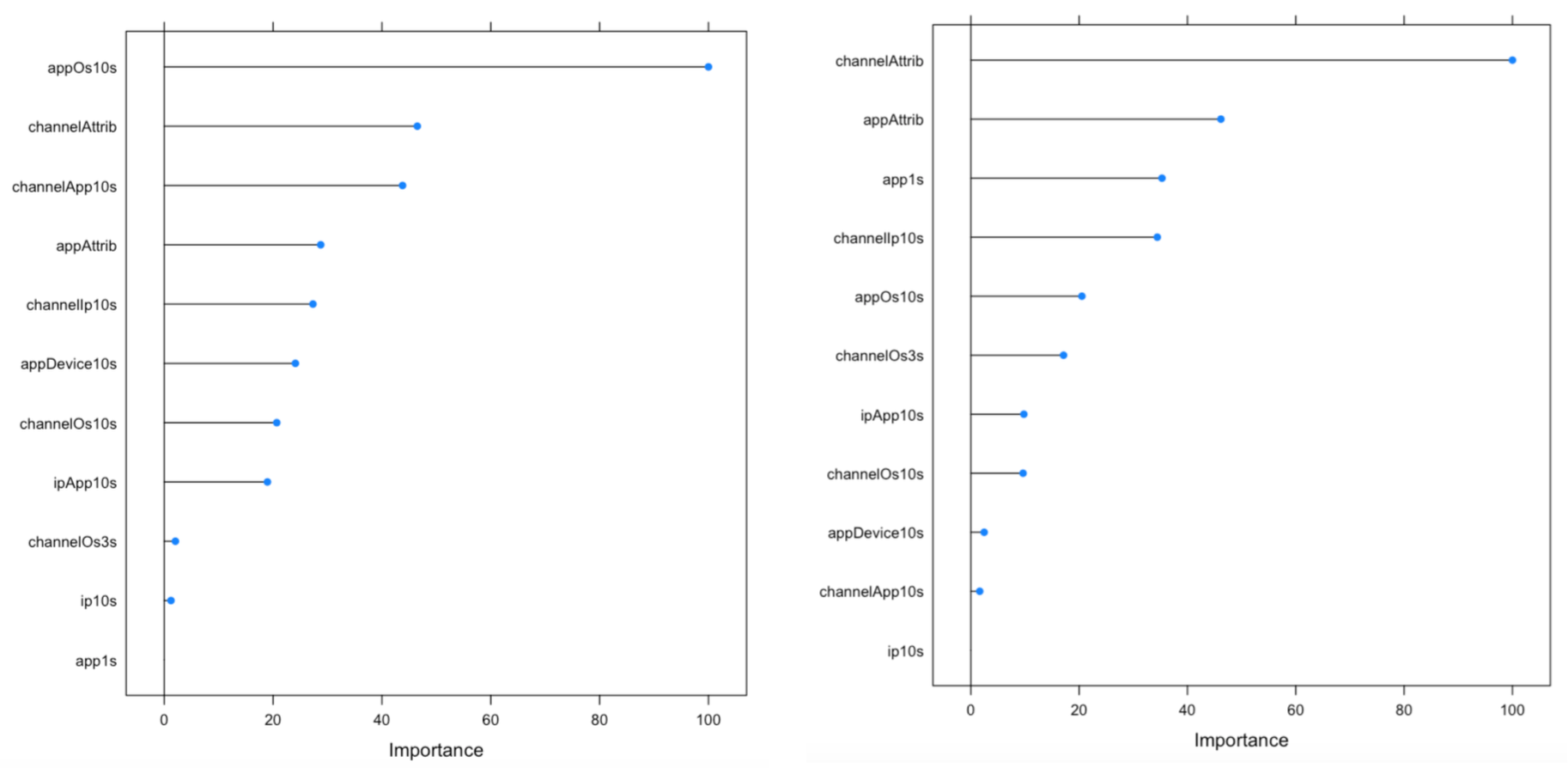
We analyzed variable importance using both baseline models as follows:
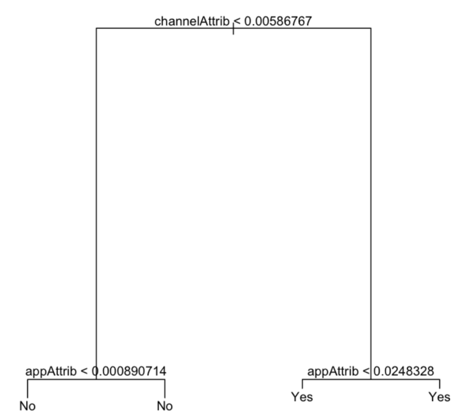
After analyzing our baselines, we built a classification tree to predict each observation belongs to the most commonly occurring class of training observations in the region to which it belongs. We use recursive binary splitting to grow a classification tree. The main purpose for building a decision tree model in this project is to visualize the decision making in which we can see channelAttrib and appAttrib are the most significant predictors.
We decided to use AUC (Area Under the Curve) and sensitivity as our metrics or the measure of goodness. From the perspective of business owners, high sensitivity means the model will maximize the proportion we can predict right among the real downloads.
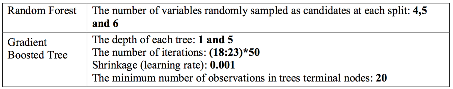
After analyzing baselines and a classification tree, we built two non-linear models: random forest and gradient boosting trees. We performed the five-fold cross validation to tune the parameters of both non-linear models as show in the table below.
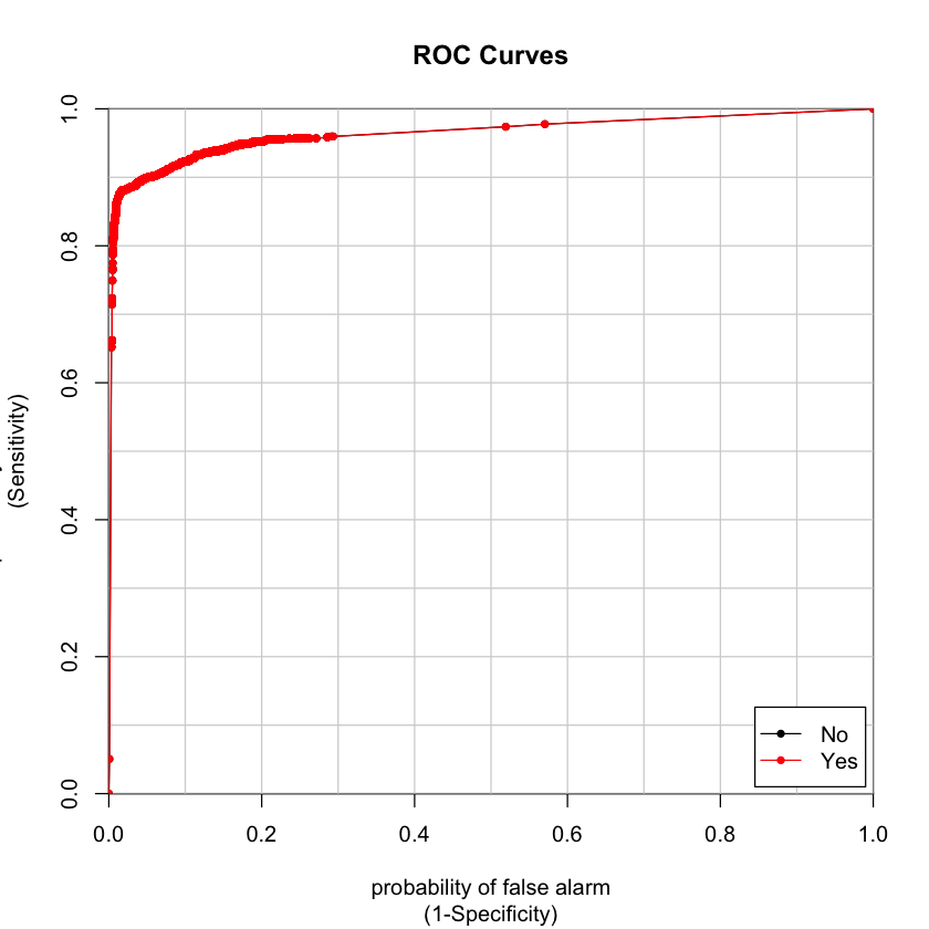
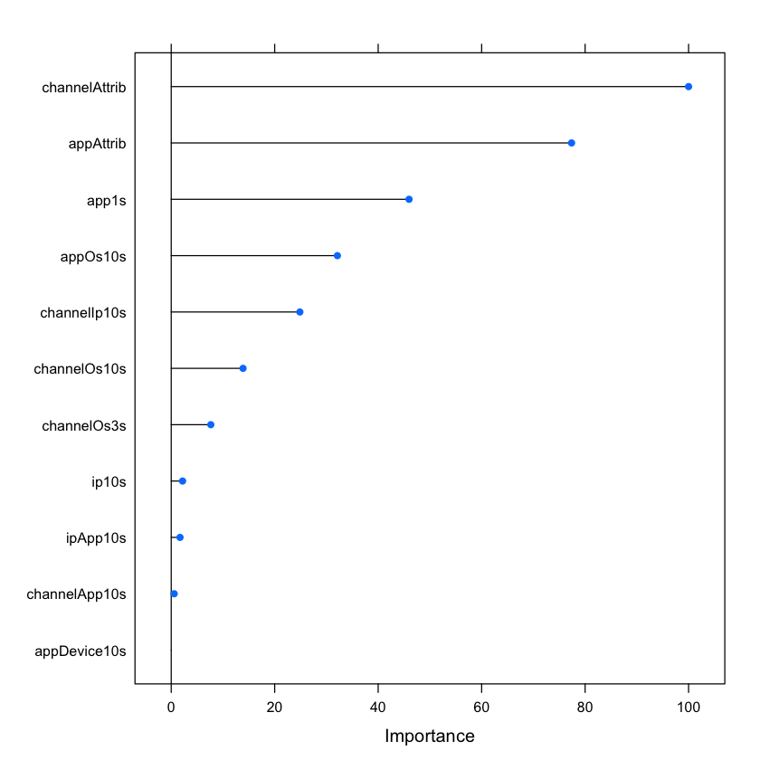
After running both non-linear model, we found that our random forest model generates highest AUC as our best model. It gives 96.36% AUC as shown in figure below and 86.26% sensitivity. The variable importance of our best model is also shown below.
Summary of The Results
We built two baseline models, a decision tree to visualize decision making process and two non- linear models to boost performance. We chose sensitivity as a supplement metric to customer appointed metric AUC for its interpretability.
Sensitivity can be intuitively interpreted as the proportion of downloads captured among all true downloads in our business scenario. However, the drawback of sensitivity alone as a metric is that a model can easily achieve 100% sensitivity if it predicts every dependent variable as positive. To avoid being trapped by this fact, we used accuracy as the objective in cross validation to tune parameters for non-linear models. Model performances are shown below.
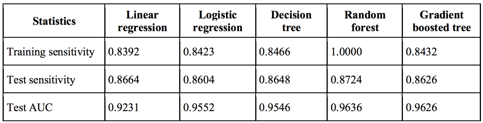
Random forest stands out as the best model in terms of both test sensitivity and test AUC. We can expect to have 87% real downloads captured by this model. However, there is an erratic pattern in this table that test sensitivity seems to outperform training sensitivity. We incline to attribute this phenomenon to test set data distribution.
In addition to model performance, we also wanted to explore what variables contributed more to the models. From the table below, we compared variable importance by models.
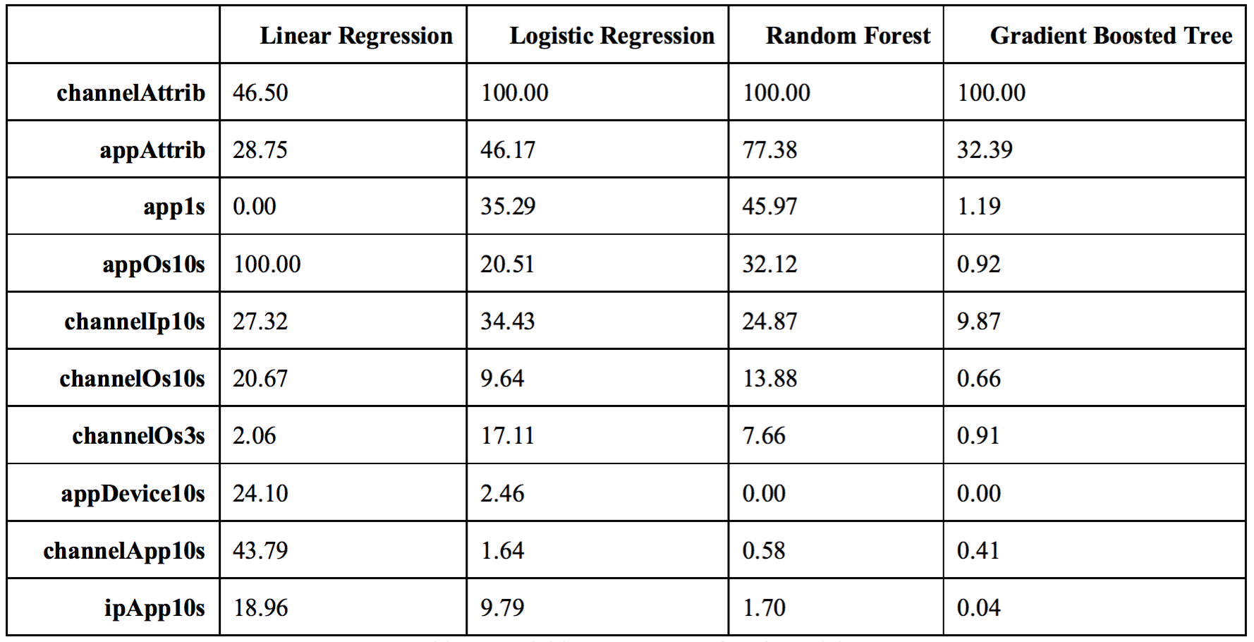
We can conclude that except for linear regression, which used t-statistics to measure variable importance, channelAttrib is the most important variable and appAttrib is the second most important.
Business Interpretation
In conclusion, the chosen model successfully predicts downloads, mainly relying on two variables: channelAttri and appAttri. The model can be used by both business owner and advertising agency such as Google AdWords and Facebook Ads.
The model enables business owners to predict downloads and manage inventory. Business owners care about user acquisition. Once the clicks happen, business owners will be able to how many new users are coming to their apps. They can make business strategy based on that analysis to manage inventory and promote sales in a more efficient way.
For advertising agencies, they can use the model to evaluate target advertising efficiency, which is directly related to their profits. In addition, advertising agencies they are able to tell which clicks are mostly likely fraudulent, so they may start investigating to protect their clients.
There is a limitation regarding to the model. The model heavily relies on two aforementioned variables because they are too useful. Once the two variables are not available, in some cases, the model is supposed to have a weak performance.