Optimizing Capacity Expansions for an Online Retailer

photo by bramwith consulting
Programming Language: Python

Problem Statement

Trojan E-commerce (not the real name, due to confidentiality), an online retailer with 17 fulfillment centers (FC) scattered centers across the US decided to build small-scale capacity expansions at a few of its FC in this fiscal year. However, as a company that prides itself in operational efficiency, Trojan wants to make sure to place the investment where it is needed the most. I have been assigned the task of identifying the top five fulfillment centers in which a small-scale capacity expansion would yield the greatest cost savings to Trojan’s supply chain.

Project Description

After much data cleaning and exploratory analysis, I decided to focus on minimizing the weekly outbound shipping cost from the fulfillment centers to customers. Trojan uses UPS 2-day delivery. Based on a regression analyses, I found that the variable component of shipping cost per item is roughly:

$1.38 x (Distance travelled in thousands of miles) x (Shipping weight of item in lbs)

The objective to minimize is the sum of the above for all items shipped in a week.

Trojan is committed to satisfying all customer demand for all of the items at all demand regions, but it can choose how many units of each item to ship per week from each fulfillment center (FC) to each demand region. Using a closer FC would reduce the shipping cost, but capacity at each FC is limited. Since Trojan replenishes inventory every week, the amount of capacity required at a FC for each item is:

(# units of the item shipped per week from the FC to all demand regions) x (Storage size of the item in cubit feet)

The sum of this across all items must not exceed the total capacity of the FC (also in cubit feet).

To identify the top candidates for capacity expansion, I decided to conduct the following analysis:

1. Formulate a Linear Programming (LP) to minimize total transportation cost for all items, subject to not exceeding the total capacity at each FC and fulfilling the weekly demand for each item from every region.
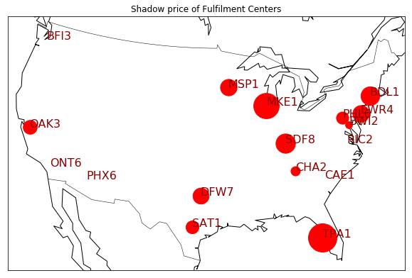
2. Use the shadow price of capacity constraints to identify the top five FCs in which a small-scale capacity expansion would yield the greatest savings to weekly transportation cost.

Understanding the Data

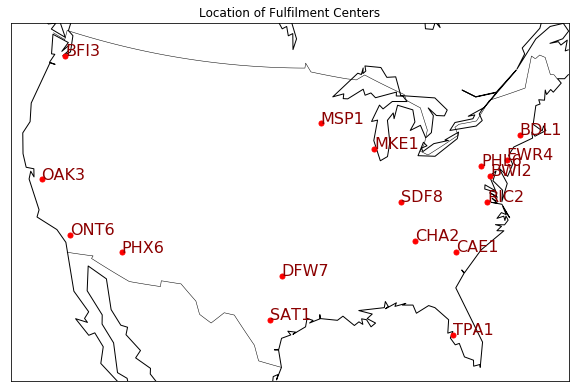
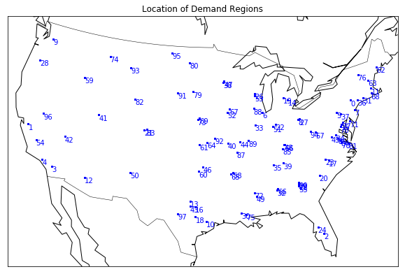
To Inspect the data, I have produced the following visualizations of these data files. After importing related files, I created the map of the fulfillment centers and the demand regions.

import matplotlib.pyplot as plt
from mpl_toolkits.basemap import Basemap
plt.figure(figsize=(10,8))

map = Basemap(llcrnrlon=-119,llcrnrlat=22,urcrnrlon=-64,urcrnrlat=49,
        projection='lcc',lat_1=33,lat_2=45,lon_0=-95)
map.drawcountries()
map.drawcoastlines()

for fc_name in centers.index:
    x,y=map(centers.loc[fc_name,'long'],centers.loc[fc_name,'lat'])
    plt.plot(x,y,'ro',markersize=5)
    plt.text(x,y,fc_name,fontdict={'size':16,'color':'darkred'})
plt.title('Location of Fulfilment Centers')
plt.show()

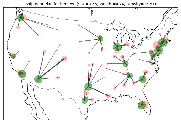
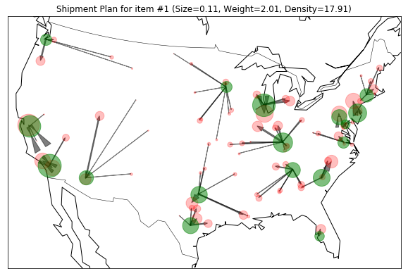
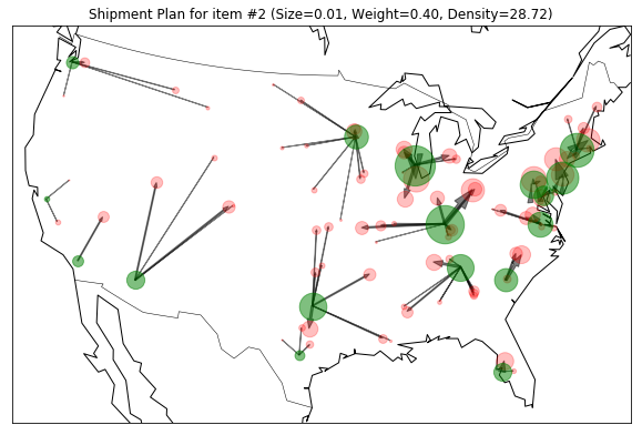
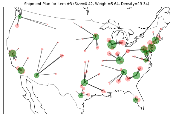
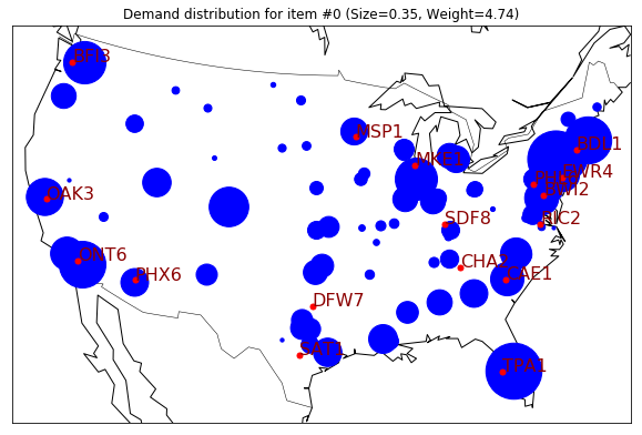
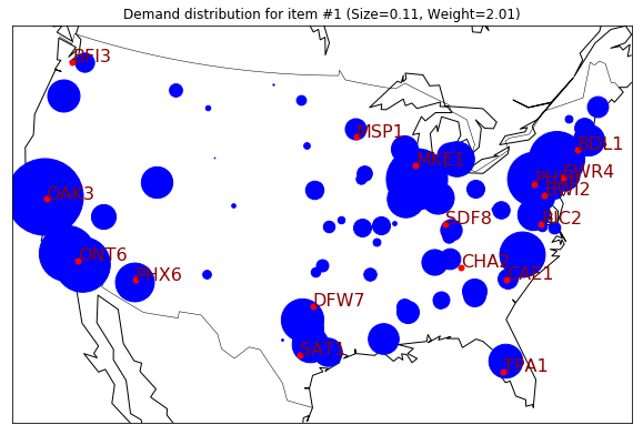
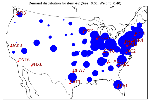
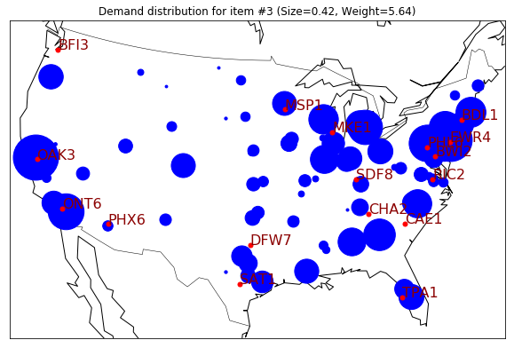
Since there are 99 combinations of the weekly estimated demand for each of the representative items, I put only the first four shipment plans to shorten the length of this portfolio.

Optimization Model

a. Define Dictionaries

First, I need to put observations in each dataframe into a dictionary. There are three dictionaries: caps, weights, and storages.

caps = {}
for a in fcs.index:
    caps[a] = fcs.loc[a,'capacity']

Iights = {}
for a in items.index:
    Iights[a] = items.loc[a,'shipping_Iight']

storages = {}
for a in items.index:
    storages[a] = items.loc[a,'storage_size']

I = distances.columns
J = distances.index
K = demands.index

b. Build the Model

#Call the gurobi model
mod=grb.Model()
x={}

for i in I:
    for j in J:
        for k in K:
            x[i,j,k]=mod.addVar(lb=0,name='x[{0},{1},{2}]'.format(i,j,k))

#Set objective function (minimize the cost)        
mod.setObjective(sum(1.38*distances.loc[j,i]*Iights[k]*x[i,j,k] for i in I for j in J for k in K),
                 sense=grb.GRB.MINIMIZE)

After defining two constraints: Fulfillment Capacity (FC) and Region Demands, I run the model to find the optimal objective (minimum supply chain cost).

#FC capacity
q = {}
for i in I:
    q[i] = mod.addConstr(sum(storages[k]*x[i,j,k] for k in K for j in J)<=caps[i],name='Capacity of {0}'.format(i))

#Region demands
for k in K:
    for j in J:
        mod.addConstr(sum(x[i,j,k] for i in I)>=demands.loc[k,j],name='Demand of {0} from {1}'.format(k,j))

mod.setParam('OutputFlag',False)
mod.optimize()

print('Optimal objective: {0:.0f}'.format(mod.ObjVal))

Optimal objective: 9841229

Optimization Output

From the table below, the top five fulfillment centers in which a small-scale capacity expansion would yield the greatest cost savings to Trojan’s supply chain are:

1. TPA1
2. MKE1
3. SDF8
4. BDL1
5. EWR4

outTable=[]
for i in q:
    outTable.append([i,q[i].PI])
outDf = pd.DataFrame(outTable,columns=['FC Name','Shadow Price'])
outDf.sort_values(by=['Shadow Price'])

	FC Name	Shadow Price
14	TPA1	-5.333088
12	MKE1	-4.276396
8	SDF8	-2.486980
5	BDL1	-2.302010
11	EWR4	-1.807986
10	MSP1	-1.798476
3	DFW7	-1.692746
15	OAK3	-1.276992
0	SAT1	-1.101105
16	PHL6	-0.984148
9	CHA2	-0.568639
13	BWI2	-0.312964
6	RIC2	0.000000
4	BFI3	0.000000
2	ONT6	0.000000
1	PHX6	0.000000
7	CAE1	0.000000

Visualizing output

Using the same method when visualizing the input data, I plotted the weekly estimated demand for each of the representative items, I put only the shadow price of each region and the first four shipment plans to shorten the length of this portfolio.

Reference

1. Linear Programming
2. Gurobi Python